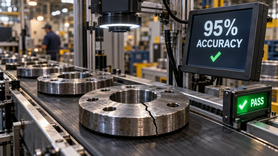
At a meeting, the supplier says, “Our defect detection system has reached 95 percent accuracy.” It sounds promising. The production manager thinks about reducing scrap, the finance manager about return on investment, and purchasing about a figure that can go into the contract.
But we still do not know whether the system will help the factory. We do not even know whether it finds defects.
Suppose a shift produces 10,000 parts: 9,500 good parts and 500 defective ones. A system that calls every part “good,” without looking at a single image, would be correct 95 percent of the time. Yet it would not find a single defective part.
Before accepting the 95 percent figure, we need to ask: 95 percent of what, on which parts, under which conditions, and with what consequences?
All numbers in this article are hypothetical and used to explain the problem. They are neither results from a real factory nor proposed acceptance limits.
Two systems with the same score and different results
Give the same 10,000 parts to two systems. System A calls every part good. System B finds some of the defects, but sometimes raises an alarm on a good part too.
| Result on 10,000 parts | System A | System B |
|---|---|---|
| Defective parts correctly detected | 0 | 400 |
| Defective parts incorrectly passed as good | 500 | 100 |
| Good parts incorrectly flagged as defective | 0 | 400 |
| Good parts correctly passed | 9,500 | 9,100 |
| Total correct classifications | 9,500 | 9,500 |
| Overall proportion correct, or Accuracy | 95% | 95% |
System B has found 400 defective parts, but it has also flagged 400 good ones. System A has raised no alarms and missed every defect. The identical figure in the sales presentation has two very different meanings on the line.
These four counts are usually presented as a confusion matrix. They are a better starting point for evaluation than a percentage on its own. A factory manager does not need to be a machine learning specialist to ask how many defective parts got through and how many good parts were set aside unnecessarily.
A missed defect and a false alarm have different consequences
Recall, or the defect detection rate, tells us what share of the truly defective parts were found. For System B, that is 400 out of 500, or 80 percent.
Precision, or the share of alarms that are correct, tells us how many parts flagged as defective actually had a defect. System B raised 800 alarms and 400 were correct, giving a precision of 50 percent.
The false alarm rate has a different denominator: 400 good parts out of 9,500 good parts, or about 4.2 percent. “Half the alarms are wrong” does not mean “half the good parts were wrongly rejected.” Google’s classification evaluation guide explains these metrics and their denominators.
For quality assurance, a defective part that gets through may lead to a return, rework or an accident. For production, a false alarm may create extra inspection, wasted material or a line stoppage. Calling both outcomes “one error” does not give them the same cost.
The type of defect matters too. A cosmetic scratch and a crack that threatens product safety should not disappear into an average. A system that finds common, straightforward defects may still struggle with a rare, critical one. The report should show each important defect group separately. If there are too few examples of a defect, the result is “insufficient evidence.”
Turn the percentage into cost and review capacity
Continuing the example, suppose the expected cost of each defective part that gets through is one million Iranian tomans, and each false alarm adds 20,000 tomans. Counting only those two items, System A costs 500 million tomans. System B costs:
100 missed defects × 1,000,000 tomans + 400 false alarms × 20,000 tomans = 108 million tomans.
Both systems had 95 percent accuracy, but these two kinds of error did not have the same cost. This calculation does not yet justify a purchase. We have left out equipment, maintenance, handling correctly detected defects and changes to the process. System A is also just an example that exposes the weakness of the metric; a proposed system should be compared with the factory’s current inspection method.
We also need to count the work. If each of System B’s 800 alarms needs 30 seconds of human review, the reviews take six hours and 40 minutes of net working time. Correct alarms can need confirmation too. This calculation also leaves out moving parts, recording decisions and alarms piling up at peak production.
“A person makes the final decision” is practical only when that person has the time, tools and authority to do it. Adding a review step to a process diagram does not create review capacity.
For defects that affect safety, a lower average cost is not enough either. Acceptable limits and controls must reflect the consequences of that particular defect. Savings on hundreds of minor errors do not justify ignoring a critical risk.
What data produced the score
A folder of clear images of good and defective parts does not necessarily represent the production line. The test scope should specify the products, lighting, conveyor speed, raw materials, camera condition and shifts covered. A score measured on one product family does not apply automatically to every product the factory makes.
First, define what is being counted. Ten images of one part are not ten independent parts. A model that performs well on individual images may fail when combining them or assigning the decision to the right physical part. The final factory metric should be close to the decision the process needs, such as accepting or diverting each part.
Test data must also be independent. If very similar images of the same part appear in both training and testing, the result can be too optimistic. Depending on the application, data may need to be separated by part, production batch or time. The final test set must not be used to tune the model or choose the threshold. The scikit-learn documentation on data leakage explains this problem.
The mix of data must be clear as well. A test set deliberately made half defective can help assess different kinds of defect. Its precision and human review workload, however, cannot be transferred directly to a line where only five percent of parts are defective.
Ask for the relevant sample count alongside every percentage. Finding all five examples of a rare defect does not provide the same evidence as a broad, varied test. Thousands of good parts do not make up for too few examples of that defect. The report should explain uncertainty and gaps in coverage. Seeing no errors in a test is not a guarantee of error-free operation.
Finally, what establishes whether a part is good or defective? One inspector’s judgment, agreement among experts, a measurement instrument or a specialist test? If experts disagree about borderline cases, the method for resolving that disagreement should be settled before evaluation. Extra decimal places do not make a percentage based on uncertain labels more reliable.
The decision threshold matters
Many models produce a score, and the system uses a threshold to decide whether a part is suspicious. For a fixed model and dataset, lowering the threshold can find more defects while also producing more false alarms. The performance report should therefore record the threshold used.
In our example, it might be possible to miss fewer defects at the cost of sending more parts to the operator. The appropriate tradeoff depends on the consequences of an error and the factory’s capacity. The threshold should not be adjusted repeatedly after seeing the final test results just to obtain a percentage that satisfies the contract.
The model version, threshold and permitted scope of use should be clear. Changing any of them may require another evaluation. An unchanged overall Accuracy does not show that the distribution of errors has stayed the same.
A correct model decision can still fail on the line
Suppose the model correctly spots a defect, but the answer arrives after the part has passed the diversion mechanism. Or an image identifier gets matched to the neighboring part. In both cases, the model can perform well in an image test while the line performs poorly.
Acceptance testing should cover the whole path: image capture, processing, decision transmission, the diversion actuator and recording the result. Peak-load latency, parts with no image and late decisions also belong in the report. Excluding them from the evaluation denominator hides some of the operational failures.
The response to a camera, network or processing failure should be defined in advance too. Continuing production, temporarily diverting parts, using alternative inspection or stopping the line are decisions that depend on risk and the process. Automatically stopping the line is not always appropriate; letting parts pass unnoticed is not a neutral choice either.
Deployment can begin in shadow mode: the system makes predictions but does not control the line. With sufficient evidence, it can move to assisting decisions and then to limited automation. At each stage, measure both model performance and the outcome of the complete process. Adding an operator or actuator changes that outcome and needs its own evaluation.
What to ask for instead of at least 95 percent accuracy
Agree on acceptance criteria before the final test. Turn these questions into the technical specification, rather than relying on one percentage:
| Area | What needs to be clear |
|---|---|
| Objective and baseline | What problem should improve, and how does the current method perform and what does it cost? |
| Scope | Which products, defects, lines, speeds and environmental conditions are covered? |
| Data and reference | How independent is the test, how many examples of each defect does it contain, and how are labels verified? |
| Errors | What limits on missed defects and false alarms apply to each important group? |
| Decision | Which model version and threshold are tested, and what approval is needed to change them? |
| Operations | What latency is acceptable, how much human review capacity is available, and what happens during a failure? |
| Acceptance and continued operation | What evidence allows deployment, and what deterioration triggers investigation, restrictions or rollback? |
A general article cannot supply the numerical limits for these conditions. Quality, production, safety and technical teams should set them using the risks, data and operational capacity of that factory. Acceptance should depend on meeting the conditions together; improving one metric should not hide the failure of another essential one.
Evaluation continues after handover. A change in material supplier, lighting or product can introduce conditions absent from the initial test. The Measure section of the NIST AI Risk Management Framework Playbook also emphasizes evaluation in the context of use and monitoring after deployment. For a factory, that means assigning responsibility, setting alarm limits and defining actions. A dashboard alone is not enough.
During monitoring, do not inspect only the parts that triggered alarms. To estimate missed defects, also sample accepted parts under an appropriate inspection plan. Otherwise, the system may seem quieter simply because it is missing more defects.
The next time a supplier says “the system has 95 percent accuracy,” ask them to express that figure in the language of the production line: how many defects get through each shift, how many good parts are flagged, how many hours of work are added for the operator, and under what conditions those estimates hold.
With clear answers, the percentage helps a decision. Without them, we still do not know what the factory is going to receive.