
From time to first token to token generation speed: how memory, concurrency and communication shape real inference performance
An inference system can produce more tokens per second while making the user wait longer for a response. It may even start writing sooner and finish later. These differences are not contradictions; they come from measuring different things under the shared label of “speed.”
The previous article, “INT8 or FP8: what your GPU can actually run”, examined why the performance listed in hardware specifications is not necessarily available in a model’s actual execution path. Here we go a step further: even when a model uses the right kernel and hardware acceleration, the card’s compute performance still cannot predict a service’s response time.
Infrastructure selection requires knowing which time must be reduced, how many concurrent requests must meet that target, and what achieving it will cost. This article, the second in this sequence within the GPU selection and AI infrastructure collection, examines that relationship.
When we say “fast,” what are we measuring?
A user sends a request, waits, sees the first part of the response, and then receives the rest. That experience involves at least two distinct timing measures: the wait before the response starts and the intervals at which subsequent parts are produced.
| Metric | Operational definition | Purpose |
|---|---|---|
| TTFT: time to first token | Time from sending the request to receiving the first content token | Measure the initial wait |
| TPOT: time per output token | Average time to produce tokens after the first token | Measure the pace of the continuing response |
| ITL: inter-token latency | Intervals between arrivals in the output stream, accounting for the number of tokens per chunk | Detect pauses and variability |
| Per-user token rate | Number of tokens after the first, divided by the time taken to receive them | Measure generation speed for one request |
| Aggregate output throughput | Total output tokens during the measurement interval, divided by its duration | Measure total service capacity |
| End-to-end latency | Time from sending the request to receiving the last token | Measure response completion time |
This distinction is consistent with inference benchmarking tools, but each tool’s precise definitions should accompany the results. Some tools measure the interval between response chunks, and each chunk may contain several tokens. GenAI-Perf metric documentation
In this article, let be the request submission time, the arrival of the first token, the arrival of the last token, and the number of output tokens:
For this request and this measurement convention, the per-user generation rate is therefore the reciprocal of TPOT. However, the reciprocal of the mean TPOT across several requests is not necessarily equal to their mean generation rate.
Client-side TTFT is not just GPU execution time: it also includes queuing, networking and request processing. In reasoning models, the first reasoning token may arrive much earlier than the first part of the final answer. AIPerf provides a separate “time to first non-reasoning output token” metric for this distinction. AIPerf metric definitions
Consequently, “a response in half a second” is incomplete without specifying where the measurement ends.
Starting sooner does not guarantee finishing sooner
Consider two hypothetical configurations:
| Configuration | TTFT | TPOT | Generation rate after the first token | Completion of a 101-token response | Completion of a 1,001-token response |
|---|---|---|---|---|---|
| A | 0.4 s | 40 ms | 25 tokens/s | 4.4 s | 40.4 s |
| B | 1 s | 20 ms | 50 tokens/s | 3 s | 21 s |
These figures are illustrative and do not represent specific hardware. They assume equal output lengths and that the stated TPOT values hold at both lengths. Completion time is calculated as:
Configuration A starts sooner; configuration B finishes long responses sooner. In this example, both finish a 31-token output at the same time; beyond that, B takes the lead.
This distinction matters when defining requirements. For a short answer, the initial wait may be the main concern. For report generation or a chain of dependent calls, completion time becomes more important. In an agentic system, the number of steps, the output length of each step and tool execution times must also remain in the calculation. Faster token generation does not shorten every part of the process.
Inference is not a uniform workload
In a typical autoregressive language model, prefill processes the input and stores the attention layers’ key and value information in the KV cache. Its output is also used to select the first token. Decode then continues generation using the previous state and extends the KV cache.
During prefill, many input tokens can participate in matrix computations. In conventional decode, each request advances by one token per step, so the opportunity to use compute units simultaneously differs. Small-batch decode can be sensitive to reading weights and the KV cache, whereas long prefill usually offers more opportunity to exploit compute capacity. This is a tendency: context length, model architecture, batch size and execution method can change the bottleneck. Transformer inference analysis in How To Scale Your Model
A good result for processing long inputs therefore does not necessarily mean faster generation for one user. A benchmark that reports only the combined total of input and output tokens may also show a larger number as input length increases, without making the continuing response any faster for the user.
Memory is more than a place to fit the model
Memory evaluation requires three separate questions: does the data fit, at what rate can it be read, and how long does it take to access the data needed?
More capacity can accommodate a model, a longer context or more active requests. Capacity alone, however, does not reduce the time needed to read the weights. Bandwidth describes a transfer rate and is not the same as access latency.
For an operation, an initial approximation is:
Here, is the number of computational operations, the compute rate, the volume of data exchanged with the memory level being examined, and that level’s bandwidth. The approximation assumes computation and transfer can overlap; execution overhead and insufficient parallelism can increase the time. NVIDIA’s guide to compute, memory and latency limitations
If data reads dominate the critical path, doubling matrix multiplication performance does not necessarily halve operation time.
For example, suppose a decode step must read exactly 70 GB of data from memory, with an effective bandwidth of 2 TB/s. Using decimal units, the lower bound for that read alone is 35 milliseconds:
This is not a speed prediction for a 70-billion-parameter model. It makes a specific assumption about the actual volume read in each step and does not separately account for attention, communication or overhead. Its value is to illustrate a limit that higher FLOPS alone cannot remove.
The KV cache must also be included in the memory budget. With conventional full-context attention, its requirements grow with sequence length and the number of active requests. Quantizing the cache or offloading it to host memory can reduce GPU memory use but has performance implications of its own; attention type and cache strategy also matter. Transformers guide to KV cache strategies
Fitting the weights does not demonstrate serving capacity.
Why can higher aggregate capacity slow down each user?
Running several requests in a batch can improve the use of weights and compute resources. Yet a system may aim to maximize aggregate output even if the interval between tokens increases for each request.
To clarify the difference, consider a steady, entirely hypothetical interval in which all requests are decoding:
| Case | Active decoding requests | Rate per request | Aggregate output rate |
|---|---|---|---|
| A | 20 | 80 tokens/s | 1,600 tokens/s |
| B | 100 | 30 tokens/s | 3,000 tokens/s |
Case B produces roughly 1.9 times as many tokens overall, but each user in case A receives output about 2.7 times faster. This table illustrates the arithmetic of a hypothetical situation, not a law describing how speed changes with concurrency.
In a real service, requests continually arrive and depart and have different lengths. Scheduling matters too. For example, vLLM documentation explains how chunked prefill divides long inputs into smaller pieces and schedules them alongside decode. Changing the scheduler’s token budget can alter the trade-off between TTFT and inter-token latency. vLLM optimization documentation
Two benchmarks using the same hardware and model but different scheduling policies can therefore produce different user experiences.
LPX: dividing the work even within decode
In the announced Vera Rubin architecture with Groq 3 LPX, NVIDIA assigns prefill and decode attention to the GPU, and decode FFN/MoE operations to the LPU. The entire decode phase is therefore not moved to the LPU. Intermediate data is exchanged between the two sides. NVIDIA’s architecture explanation
The diagram below is a conceptual reconstruction of that division of work. It omits subsidiary operations such as normalization, residual connections and tensor distribution details:
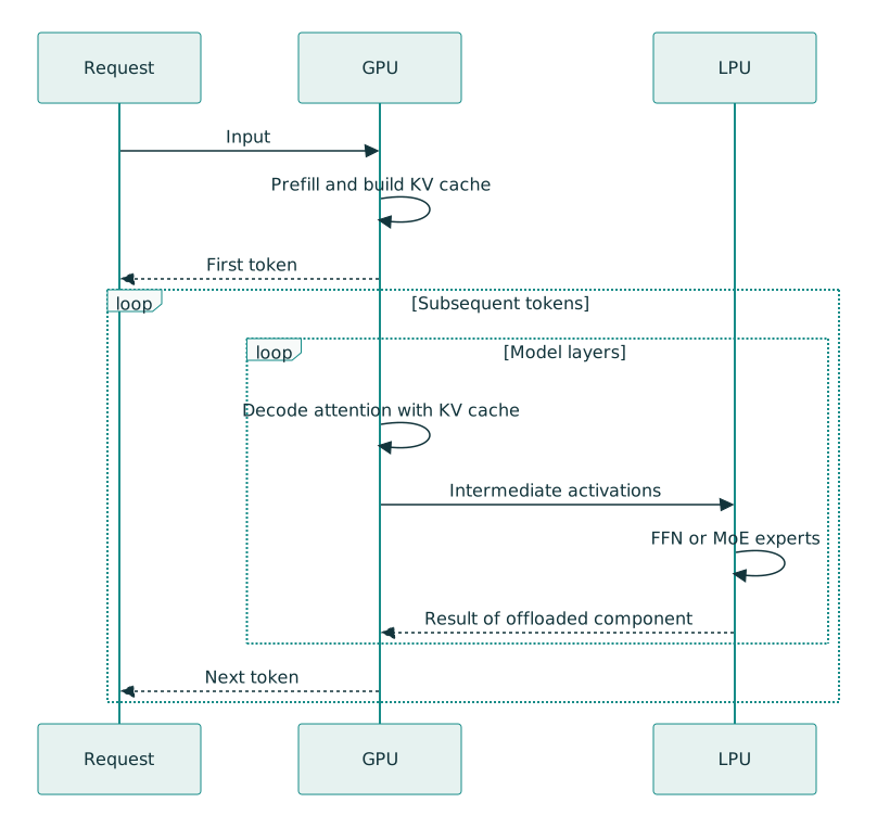
Download the diagram’s Mermaid source
This is different from separating prefill and decode into two processor groups. DistServe is an example of disaggregating the two phases to control interference and optimize serving under latency constraints; LPX extends the division to components within decode itself. Original DistServe paper
The reason to examine this example is architectural, rather than its product name: different parts of a request do not need the same proportions of memory capacity, bandwidth and compute performance.
Read memory figures at the correct scale
The official LPX page lists these specifications:
| Announced specification | Scale |
|---|---|
| 500 MB of SRAM | Per LPU |
| 150 TB/s of SRAM bandwidth | Per LPU |
| 256 LPU chips | One LPX rack |
| 128 GB of SRAM and 12 TB of DDR5 | One LPX rack |
| Approximately 40 PB/s of SRAM bandwidth | Aggregate across the rack |
| 640 TB/s of scale-up bandwidth | Rack level |
Source: Official NVIDIA Groq 3 LPX page
These are vendor-announced specifications. A rack’s aggregate SRAM bandwidth cannot be compared directly with the HBM bandwidth of a single GPU. DDR5 capacity is not SRAM capacity, either, and the intra-rack scale-up rate does not determine the usable rate of a particular GPU-to-LPU exchange.
Nor does a total of 128 GB of SRAM establish that all the weights of a very large model always fit in SRAM. Data placement, distribution and how often data moves must remain part of the analysis.
Communication determines the cost of dividing the work
Splitting an operation between two accelerators is beneficial when the execution savings exceed the additional transfer and coordination costs.
A transfer’s duration can be approximated as:
Here, is the fixed startup and delivery latency, the message size, and the path’s effective bandwidth. This simple model does not fully capture congestion or runtime variability, but it makes one distinction clear: for small messages, reducing fixed latency may matter more than increasing bandwidth.
For example, suppose a hypothetical design requires 80 dependent round trips to generate each token, and the total fixed cost of each round trip is 10 microseconds. The fixed communication contribution, before accounting for data volume, is 0.8 milliseconds. At 50 microseconds per round trip, it rises to 4 milliseconds.
This example is not an LPX specification. It shows why even small exchanges can matter in a frequently repeated loop.
Without overlap, a simple condition for offloading a component to be beneficial is:
In a real implementation, the relevant costs are those that remain on the critical path after overlap.
The same consideration applies to adding GPUs. Increasing tensor parallelism can free up more memory, but requires more coordination; vLLM documentation explicitly notes this overhead. vLLM parallelism considerations
Thus, “the model runs on four cards” does not mean “each user gets a response four times faster.”
What are the limits of a vendor’s claim?
For the combination of Vera Rubin NVL72 and LPX, NVIDIA claims up to 35 times more throughput per megawatt than GB200 NVL72 at approximately 400 tokens per second per user. This is a vendor claim about the configuration and scenario presented; it does not mean a 35-fold reduction in every request’s response time or universal LPX superiority. NVIDIA’s chart and explanation
Before using such a claim for procurement, the model, numerical precision, input and output lengths, concurrency, rack count, power measurement boundary and latency constraint must be known. A “tokens per megawatt” figure also does not by itself account for purchase price, networking costs, operations or actual capacity utilization.
Among the sources reviewed for this article, the LPX description rests on NVIDIA’s own documentation. Its figures are not presented here as independently reproduced results.
What capacity can actually be sold or used?
A service may achieve a high token rate in a benchmark while a substantial share of requests exceeds the permitted latency. That benchmark’s nominal capacity is not dependable serving capacity.
In our Targoman deployment under load (report in Persian), responses usually began in less than a second at low load; under pressure, the wait could reach the 20-second cutoff, at which point a request with no response started was cancelled. The system had roughly 300 concurrent requests during that incident, but not all completed successfully. This illustrates why usable capacity must count responses delivered within an acceptable time, rather than simply the requests present in the system.
Goodput addresses this issue by counting requests that meet specified constraints. In AIPerf, it is also distinct from the proportion of requests that comply with those constraints: a service rejecting many requests should not be judged successful simply because the remaining responses are fast. AIPerf goodput guide
For a particular service, an initial target might be: “At least 95% of requests must have both TTFT below two seconds and TPOT below 50 milliseconds.” These numbers are examples and should be derived from product requirements.
The emphasis on “both” is deliberate. Reporting the 95th percentile of each metric separately does not guarantee that the same 95% of requests meet both conditions.
Response quality also requires separate evaluation. Shortening the output or changing the model may improve timing, but a comparison remains valid only if the output still meets the application’s needs.
Define acceptance tests from service requirements
Before comparing cards, the test specification must be fixed and reproducible:
| Test area | What to record |
|---|---|
| Model and quality | Weight version, tokenizer, quantization and response acceptance criteria |
| Input and output | Length distributions, language, multi-turn context and actual output length |
| Incoming load | Arrival rate, concurrency, traffic bursts and test duration |
| Execution engine | Versions, batching, parallelism, chunked prefill and cache settings |
| Acceleration features | Whether prefix caching and speculative decoding are enabled |
| Latency | TTFT and TPOT distributions, streaming pauses and completion time |
| Capacity | Aggregate output rate, successful requests, errors, timeouts and goodput |
| Infrastructure and cost | Card and server counts, topology, power consumption and total configuration cost |
A single-user test helps establish a lower latency bound but does not determine service capacity. Increase the load and identify the point beyond which user experience constraints no longer hold. A fixed-concurrency test must also be distinguished from a fixed-arrival-rate test: in the former, a slower service can automatically delay the next request and reduce the pressure applied.
For Persian content, the sample must contain real Persian inputs. “Tokens per second” does not necessarily represent the same volume of text across two tokenizers, so comparing different models also requires assessing quality and the time taken to complete a common task.
The objective must also be explicit: isolate the hardware’s effect, or compare the best deployable service. For the former, settings should be as similar as possible. For the latter, each stack can be optimized, provided differences are documented and the quality criterion is preserved.
GPU selection starts with defining the response you need
When buying inference infrastructure, “Which card is faster?” is premature. First establish whether responses are short or long, how many concurrent requests are expected, what latency is acceptable, and which part of execution consumes the time.
LPX illustrates an architectural response to the different needs of inference components. Its existence does not imply that every service needs heterogeneous hardware. Sometimes better scheduling, the right software stack or reduced memory pressure solves the problem; sometimes dividing work between processors is worth the communication cost.
The purchasing criterion should be the capacity to serve requests at the required quality and latency. Compute, memory and networking are means to that end. Ranking higher in one of those columns alone does not establish better response performance.