Technical notes / Compute infrastructure
GPUs and AI servers: what to choose, and why?
Compare accelerators and servers, check software support and assess performance per cost, based on real workloads.
Where should I start?
Begin with the work the system needs to do. The tables help you compare options; the articles explain what the differences mean. Choose the path that matches your decision.
Which path fits my needs?
Start with the workload: the model's memory requirements, numerical format, communication pattern and service targets. Use the tables to compare hardware, then follow the guides to assess software compatibility, host resources and the full cost of deployment.
For language-model inference, compare models by memory and hardware requirements; model size, input length and concurrency determine the GPU capacity needed.
AI accelerator reference
Compare GPUs against the work they need to do
Explore cards, modules, processors, complete accelerator systems and cloud offerings for AI.
Data last reviewed8 September 2026
How to read this tableProduct type identifies cards, modules, processors, complete systems and cloud services. In the FP8 and FP16 columns, the first rate is dense and the second, where available, uses sparsity. FP32 and FP64 show general-purpose vector rates, which are not directly comparable with Tensor/Matrix AI rates; these are therefore shown separately.
Detailed filters 61 Results
Column groups:
Results61of 61 models
Largest memory480GB
Highest bandwidth80TB/s; compare memory types
Lowest power150Cloud AI 100 Ultra
| Compare | Details | Type | Workloads | ||||||
|---|---|---|---|---|---|---|---|---|---|
 Intel Intel | Card | Rack scale | Preliminary specificationsManufacturer | 480LPDDR5X; up to the announced capacity | Not published by manufacturerNo public figure | 350W | Enterprise inference | ||
 INSTINCT INSTINCT | Module | Rack scale | Preliminary specificationsManufacturer | 432HBM4 | 23.3TB/s | Not published by manufacturerNo standalone figure | HPCLarge-model trainingEnterprise inference | ||
| INSTINCT | Module | Rack scale | System onlyManufacturer | 432HBM4 | 23.3TB/s | Not published by manufacturerNo standalone figure | Large-model trainingEnterprise inferenceHPC | ||
 NVIDIA NVIDIA | Module | Rack scale | Current generationManufacturer | 288HBM3e | 8TB/s | 1,400W | Large-model trainingEnterprise inferenceHPCMulti-tenancy | ||
| INSTINCT | Module | Rack scale | Current generationManufacturer | 288HBM3e | 8TB/s | 1,000W | Large-model trainingEnterprise inferenceHPC | ||
| INSTINCT | Module | Rack scale | Current generationManufacturer | 288HBM3e | 8TB/s | 1,400W | Large-model trainingEnterprise inferenceHPC | ||
| NVIDIA | Module | Rack scale | System onlyManufacturer | 288HBM4 | 22TB/s | Not published by manufacturerNo standalone figure | Large-model trainingEnterprise inferenceHPC | ||
| INSTINCT | Module | Rack scale | Current generationManufacturer | 256HBM3e | 6TB/s | 1,000W | Large-model trainingEnterprise inferenceHPC | ||
| NVIDIA | Module | Rack scale | Current generationManufacturer | 180–192HBM3e | 8TB/s | 1,200W | Large-model trainingEnterprise inferenceHPCMulti-tenancy | ||
 Google Google | Cloud | Rack scale | Current generationManufacturer technical documentation | 192HBM; 96 GB per chiplet | 7.4TB/s | Not applicableNo standalone figure | Large-model trainingEnterprise inferenceHPC | ||
| INSTINCT | Module | Rack scale | Current generationManufacturer | 192HBM3 | 5.3TB/s | 750W | Large-model trainingEnterprise inferenceHPC | ||
| NVIDIA | Card | Rack scale | Current generationManufacturer | 141HBM3e | 4.8TB/s | 600W | Enterprise inferenceHPCMulti-tenancy | ||
| NVIDIA | Processor | Data center | Current generationManufacturer | 141HBM3e | 4.8TB/s | 700W | Large-model trainingEnterprise inferenceHPCMulti-tenancy | ||
 Qualcomm Qualcomm | Card | Rack scale | Current generationManufacturer | 128LPDDR4X | 0.5TB/s | 150W | Enterprise inference | ||
| Intel | Card | Rack scale | Current generationManufacturer | 128HBM2e | 3.7TB/s | 600W | Large-model trainingEnterprise inference | ||
| INSTINCT | Module | Data center | Previous generationManufacturer | 128HBM2e | 3.2TB/s | 560W | Large-model trainingEnterprise inferenceHPC | ||
 Huawei Huawei | Card | Rack scale | Current generationManufacturer | 112HBM | 1.4TB/s | 600W | Enterprise inferenceLarge-model training | ||
| Huawei | Processor | Rack scale | System onlyManufacturer | 96HBM | 4TB/s | Not published by manufacturerNo standalone figure | Large-model trainingEnterprise inferenceHPC | ||
| Huawei | Card | Rack scale | Current generationManufacturer | 48 or 96LPDDR4X | 0.4TB/s | 150W | Enterprise inference | ||
| NVIDIA | Card | Rack scale | Current generationManufacturer | 96GDDR7 | 1.6TB/s | 600W | Enterprise inferenceGraphics and renderingMulti-tenancy | ||
 AWS AWS | Cloud | Rack scale | Current generationManufacturer | 96HBM3 | 2.9TB/s | Not applicableNo standalone figure | Large-model trainingEnterprise inference | ||
| Google | Cloud | Rack scale | Current generationManufacturer technical documentation | 95HBM | 2.8TB/s | Not applicableNo standalone figure | Large-model trainingEnterprise inference | ||
| NVIDIA | Card | Rack scale | Current generationManufacturer | 94HBM3 | 3.9TB/s | 400W | Enterprise inferenceHPCMulti-tenancy | ||
| NVIDIA | Card | Rack scale | Previous generationManufacturer | 80HBM2e | 1.9TB/s | 300W | Enterprise inferenceHPCMulti-tenancy | ||
| NVIDIA | Processor | Data center | Previous generationManufacturer | 80HBM2e | 2TB/s | 400W | Large-model trainingEnterprise inferenceHPCMulti-tenancy | ||
| NVIDIA | Card | Rack scale | Previous generationManufacturer technical documentation | 80HBM2e | 2TB/s | 300W | Large-model trainingEnterprise inferenceHPCMulti-tenancy | ||
| NVIDIA | Card | Data center | Previous generationManufacturer technical documentation | 80HBM2e | 1.9TB/s | 300W | Large-model trainingEnterprise inferenceHPCMulti-tenancy | ||
| NVIDIA | Card | Data center | Current generationManufacturer | 80HBM2e | 2TB/s | 350W | Large-model trainingEnterprise inferenceHPCMulti-tenancy | ||
| NVIDIA | Processor | Data center | Current generationManufacturer | 80HBM3 | 3.4TB/s | 700W | Large-model trainingEnterprise inferenceHPCMulti-tenancy | ||
| Huawei | Processor | Data center | Current generationManufacturer technical documentation | 64HBM | Not published by manufacturerNo public figure | Not published by manufacturerNo standalone figure | Large-model trainingEnterprise inference | ||
| INSTINCT | Card | Rack scale | Previous generationManufacturer | 64HBM2e | 1.6TB/s | 300W | HPCEnterprise inference | ||
| NVIDIA | Card | Consumer | Current generationManufacturer technical documentation | 48GDDR6X | 1TB/s | 425W | Large-model trainingEnterprise inferenceLocal AIGraphics and renderingMulti-tenancy | ||
| NVIDIA | Card | Rack scale | Current generationManufacturer technical documentation | 48GDDR6 | 0.9TB/s | 300W | Large-model trainingEnterprise inferenceGraphics and renderingMulti-tenancy | ||
| NVIDIA | Card | Rack scale | Current generationManufacturer | 48GDDR6 | 0.9TB/s | 350W | Enterprise inferenceGraphics and rendering | ||
| NVIDIA | Card | Workstation | Previous generationManufacturer technical documentation | 48GDDR6 | 0.7TB/s | 295W | Enterprise inferenceLocal AIGraphics and renderingMulti-tenancy | ||
| NVIDIA | Card | Workstation | Current generationManufacturer | 48GDDR6 | 1TB/s | 300W | Local AIGraphics and rendering | ||
| NVIDIA | Card | Workstation | Previous generationManufacturer | 48GDDR6 | 0.8TB/s | 300W | Large-model trainingEnterprise inferenceLocal AIGraphics and renderingMulti-tenancy | ||
| NVIDIA | Card | Data center | Previous generationManufacturer technical documentation | 40HBM2 | 1.6TB/s | 250W | Large-model trainingEnterprise inferenceHPCMulti-tenancy | ||
 Tenstorrent Tenstorrent | Card | Workstation | Current generationManufacturer | 32GDDR6 | 0.5TB/s | 300W | Local AIEnterprise inference | ||
| Google | Cloud | Rack scale | Current generationManufacturer technical documentation | 32HBM | 1.6TB/s | Not applicableNo standalone figure | Large-model trainingEnterprise inference | ||
| NVIDIA | Card | Consumer | Current generationManufacturer | 32GDDR7 | 1.8TB/s | 575W | Local AIGraphics and rendering | ||
| INSTINCT | Card | Data center | Previous generationManufacturer | 32HBM2 | 1.2TB/s | 300W | Large-model trainingEnterprise inferenceHPC | ||
| AMD | Card | Workstation | Current generationManufacturer | 32GDDR6 | 0.6TB/s | 300W | Local AIGraphics and rendering | ||
| NVIDIA | Card | Data center | Previous generationManufacturer technical documentation | 16 or 32HBM2 | 0.9TB/s | 250W | Large-model trainingEnterprise inferenceHPCMulti-tenancy | ||
| NVIDIA | Module | Data center | Previous generationManufacturer technical documentation | 16 or 32HBM2 | 0.9TB/s | 300W | Large-model trainingEnterprise inferenceHPCMulti-tenancy | ||
| NVIDIA | Card | Consumer | Previous generationManufacturer | 24GDDR6X | 0.9TB/s | 350W | Large-model trainingEnterprise inferenceLocal AIGraphics and renderingMulti-tenancy | ||
| NVIDIA | Card | Consumer | Previous generationManufacturer | 24GDDR6X | 1TB/s | 450W | Large-model trainingEnterprise inferenceLocal AIGraphics and renderingMulti-tenancy | ||
| NVIDIA | Card | Consumer | Previous generationManufacturer | 24GDDR6X | 1TB/s | 450W | Local AIGraphics and rendering | ||
| NVIDIA | Card | Consumer | Current generationManufacturer technical documentation | 24GDDR6X | 1TB/s | 425W | Large-model trainingEnterprise inferenceLocal AIGraphics and renderingMulti-tenancy | ||
| Tenstorrent | Card | Workstation | Current generationManufacturer technical documentation | 24GDDR6 | 0.6TB/s | 300W | Local AIEnterprise inference | ||
| NVIDIA | Card | Consumer | Current generationManufacturer | 16GDDR6X | 0.7TB/s | 320W | Large-model trainingEnterprise inferenceLocal AIGraphics and renderingMulti-tenancy | ||
| NVIDIA | Card | Consumer | Previous generationManufacturer | 12GDDR6 | 0.4TB/s | 170W | Enterprise inferenceLocal AIMulti-tenancy | ||
| NVIDIA | Card | Consumer | Current generationManufacturer | 12GDDR6X | 0.5TB/s | 200W | Enterprise inferenceLocal AIGraphics and renderingMulti-tenancy | ||
| NVIDIA | Card | Consumer | Previous generationManufacturer technical documentation | 11GDDR6 | 0.6TB/s | 250W | Enterprise inferenceLocal AIGraphics and renderingMulti-tenancy | ||
| NVIDIA | Card | Consumer | Previous generationManufacturer | 10GDDR6X | 0.8TB/s | 320W | Enterprise inferenceLocal AIGraphics and renderingMulti-tenancy | ||
| NVIDIA | Card | Consumer | Previous generationManufacturer | 8GDDR6 | 0.4TB/s | 215W | Enterprise inferenceLocal AIGraphics and renderingMulti-tenancy | ||
| NVIDIA | Card | Consumer | Previous generationManufacturer | 8GDDR6 | 0.4TB/s | 220W | Enterprise inferenceLocal AIGraphics and renderingMulti-tenancy | ||
| Huawei | Processor | Rack scale | System onlyManufacturer | Not published by manufacturerHBM; SKU-specific capacity | Not published by manufacturerNo public figure | Not published by manufacturerNo standalone figure | Large-model trainingEnterprise inference | ||
 Cerebras Cerebras | System | Rack scale | Current generationManufacturer | Not applicableOn-wafer SRAM plus disaggregated MemoryX | Not applicableTB/s | 23,000W | Large-model trainingHPC | ||
| NVIDIA | System | Rack scale | System onlyManufacturer | Not applicableDistributed rack SRAM; 500 MB per LPU | Not applicableTB/s | Not published by manufacturerNo standalone figure | Enterprise inference | ||
 Groq Groq | System | Rack scale | System onlyManufacturer | Not published by manufacturerOn-chip SRAM; public SKU-specific capacity not published | 80TB/s | Not published by manufacturerNo standalone figure | Enterprise inference |
GPU types for AI: consumer, workstation and data center
How GPU product families differ in memory, software support and deployment requirements—and when each is a practical choice.
A GPU marketed for gaming can be useful for AI, and a data center accelerator can be an expensive way to run a small model. The product category tells us something about the intended operating environment. It does not, by itself, tell us which card will deliver the best result for a particular workload.
The term GPGPU means general-purpose computing on graphics processing units. It describes using a GPU for computation beyond graphics; it is not a separate product family. For infrastructure planning, it is more useful to distinguish consumer cards, professional workstation cards and data center accelerators.
Consumer GPUs
Consumer GPUs are designed primarily for gaming and personal computers. They can also serve development, research, inference and fine-tuning workloads that fit within their memory and software constraints. NVIDIA’s GeForce RTX range is a familiar example. AMD cards may also be suitable, but the exact GPU, operating system and required libraries must be checked against the supported software stack.
Cards such as the RTX 3090, RTX 4090 and RTX 5090 deserve consideration when the workload fits on one card or can be divided into independent jobs. In the right configuration, their performance per unit of cost can be attractive compared with older data center hardware. That comparison changes when a job requires more memory, extensive communication between GPUs or operational features that the consumer card does not provide. The method matters more than a standing recommendation for a particular model; see choosing a GPU for the workload.
A gaming card also brings mechanical and thermal requirements that are easy to overlook. Large coolers, power connectors and open-air fans can make dense server installation impractical. A chassis with enough PCIe slots is not necessarily a compatible chassis. The PCIe server selection guide explains why compatibility must be checked against the exact card and server bill of materials.
Professional workstation GPUs
NVIDIA’s professional graphics products have moved through names including Quadro, RTX A, RTX Ada and RTX PRO. AMD’s corresponding workstation families have included FirePro and Radeon PRO. These cards target applications such as visualization, engineering and content creation, with professional drivers and configurations suited to those environments.
They can also be useful for AI. The RTX A6000 and RTX 6000 Ada, for example, provide 48 GB of memory, which opens up workloads that do not fit on a smaller consumer card. A professional card may offer a more convenient form factor or a supported workstation configuration as well.
The relevant question is whether those capabilities justify the price for the intended service. Professional branding is not a guarantee of better training or inference performance per cost. Compare the exact SKU, usable memory, supported numerical formats, cooling arrangement and software path. Workstation and server editions within the same product family may differ substantially.
Data center accelerators
Data center accelerators are designed for sustained compute workloads and integration into server platforms. Depending on the product, their advantages can include high-bandwidth memory, larger memory capacity, reliability and management features, and faster communication between accelerators. Those capabilities matter for large model training, memory-intensive inference and some high-performance computing workloads.
This category includes several generations of NVIDIA accelerators, from A100 through H100 and H200 to Blackwell, as well as AMD’s Instinct family. Product specifications, supported software and server qualification must still be checked at the SKU level. A newer architecture is not automatically a better fit for an existing model or runtime.
The deployment format is another decision. Some accelerators are PCIe add-in cards; others form part of an integrated multi-GPU platform. The PCIe and SXM comparison explains how that choice affects expansion, power, cooling and communication between GPUs.
Start with the work the machine will do
For development and independent inference jobs, a consumer or workstation card may be a sensible starting point. For a model that needs more memory or spends a substantial share of execution time exchanging data between GPUs, a data center platform may justify its higher cost. In either case, the host server still needs enough CPU capacity, RAM, storage and network bandwidth to keep the accelerators busy; those requirements are covered in the server platform guide.
Buy the capabilities the workload can use. Paying for additional memory can make an otherwise impossible deployment viable. Paying for an interconnect that the software never uses adds cost without increasing useful capacity.
PCIe or SXM: choosing a GPU platform for AI
How memory, interconnects, power and expansion requirements affect the choice between PCIe cards and integrated SXM platforms.
Two systems can carry GPUs with the same family name and still behave very differently. The difference may come from the GPU variant itself, its power limit, its memory or the links connecting it to other GPUs. Comparing PCIe and SXM therefore means comparing complete configurations, not just connectors.
A card versus an integrated platform
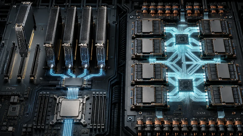
A PCIe GPU is an add-in card installed in a compatible server or workstation. SXM is NVIDIA’s module form factor for GPUs mounted on a dedicated baseboard. An SXM module cannot be inserted into a PCIe slot; it requires a platform built for that module, including its power delivery and cooling.
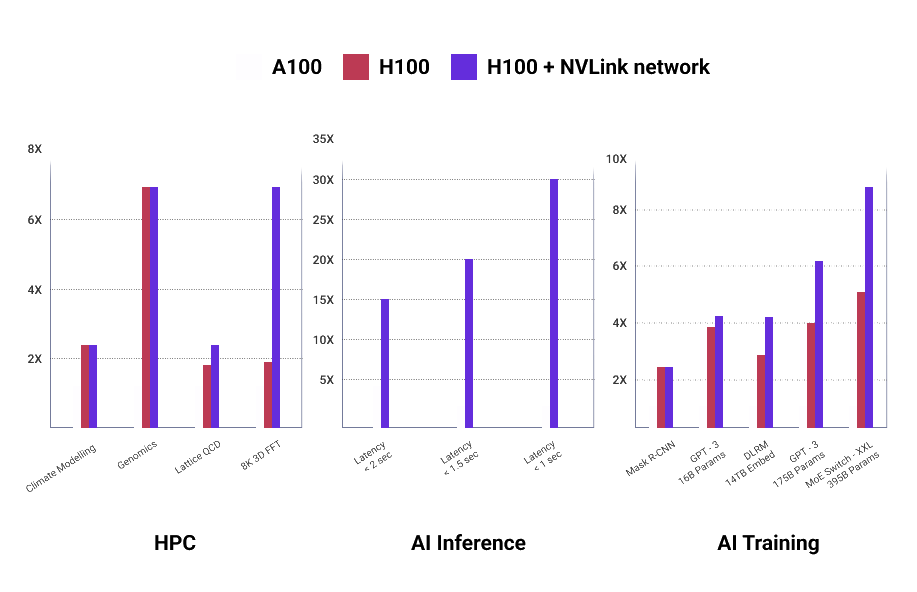
In H100 and H200 eight-GPU HGX systems, SXM GPUs communicate through NVLink and NVSwitch. This provides a high-bandwidth fabric inside the server. The value of that fabric depends on whether the workload actually moves substantial amounts of data between GPUs.
Some PCIe GPU variants also support NVLink bridges. The supported number of GPUs and bridge arrangement are specific to the product and server configuration. Do not assume that every PCIe card supports NVLink, or that a bridged pair provides the same topology as an eight-GPU HGX baseboard. For GPUs communicating over PCIe, the CPU attachment, PCIe switches and NUMA layout also matter.
When fast GPU-to-GPU communication pays off
A large model divided across multiple GPUs may require frequent communication during training or inference. In those conditions, reducing communication time can materially improve the usefulness of each additional GPU. An integrated SXM platform is worth evaluating when that communication is a measured bottleneck.
Independent jobs are different. If eight users each run a model on a separate GPU, their work may share little or no data across the GPU fabric. They can benefit from a dense server without benefiting much from NVSwitch. The DGX, HGX and PCIe server comparison separates the value of the interconnect from the value of the complete system and its support services.
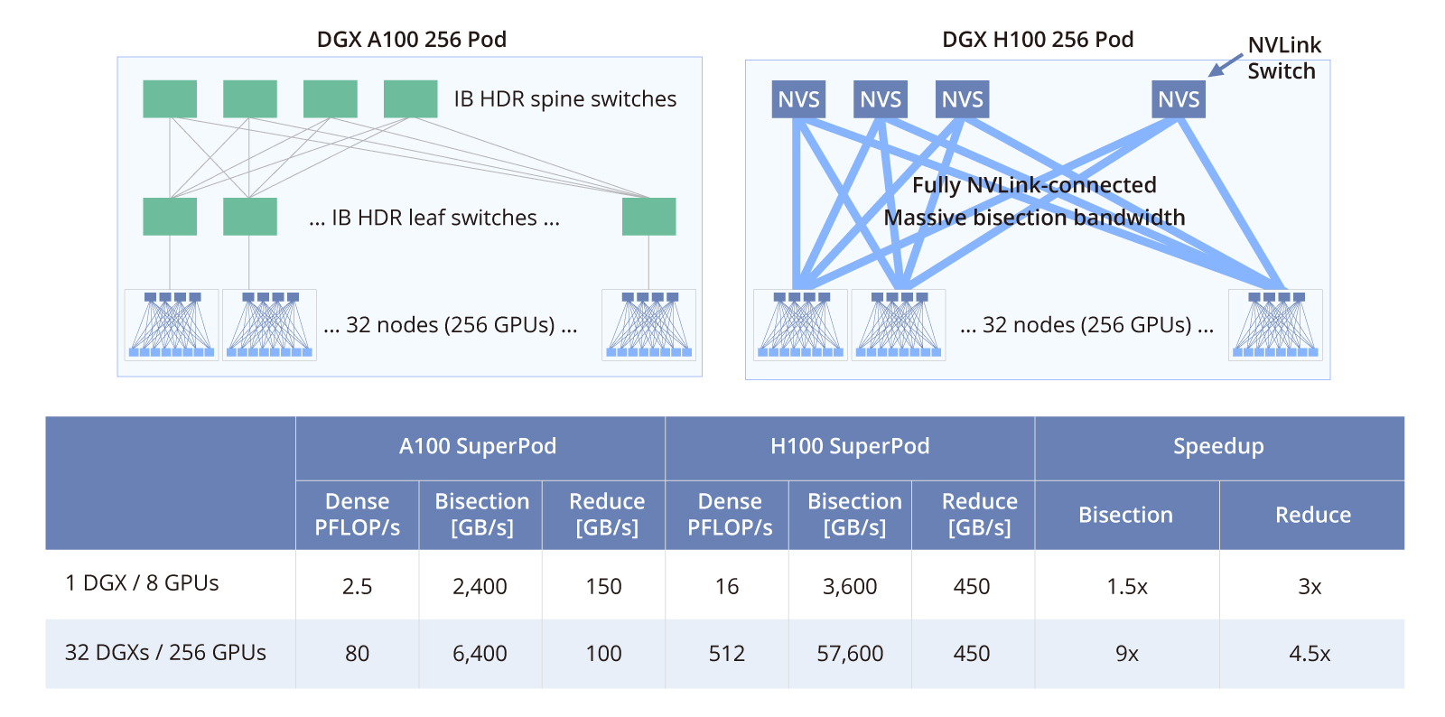
The boundary of the fabric is important. In the H100/H200 systems discussed here, NVSwitch connects GPUs within a node. Communication between servers also requires a compute network, suitable NICs and the software configuration to use them. NVIDIA’s DGX SuperPOD reference architecture describes the compute, storage and management networks separately. Rack-scale NVLink systems in other generations must be assessed against their own architecture; their topology should not be inferred from this eight-GPU example.
Expansion and utilization
A compatible PCIe server can often be purchased with fewer GPUs and expanded later. That flexibility is useful when demand grows gradually, when users need different card types or when the workload is still being characterized. Expansion still depends on the approved server configuration: power supplies, risers, cooling kits and supported GPU combinations may need to be specified at the start.
An integrated SXM system commits more of the investment at once. Standardization can simplify fleet operations, but idle GPUs and unused interconnect capacity remain real costs. Before selecting it, measure whether the target application scales effectively from one or two GPUs to four and eight.
Memory and power: compare the exact variants
The original 80 GB H100 PCIe uses HBM2e, as specified in NVIDIA’s H100 PCIe product brief. The 80 GB H100 SXM uses HBM3. The H100 datasheet lists nominal memory bandwidth of approximately 2 TB/s and 3.35 TB/s respectively. H100 NVL is another configuration again; its specifications should not be substituted for those of the 80 GB PCIe card.
The power envelope also differs: the 80 GB H100 PCIe is rated up to 350 W, while H100 SXM configurations can reach 700 W per GPU. The server must be designed for the selected operating point. These figures do not establish energy efficiency on their own. A higher-power GPU may finish a suitable task sooner, while an underutilized one may consume more energy without shortening execution enough to justify it. Measure energy and cost per completed task alongside elapsed time.
Memory capacity, memory bandwidth and compute capability can all change between variants and generations. Numerical-format support adds another layer: INT8 and FP8 support in practice explains why a hardware specification does not guarantee a usable runtime path.
Match the platform to the communication pattern
| Workload characteristic | What to evaluate first |
|---|---|
| Independent inference, development or analytics jobs | PCIe cards with sufficient memory and a suitable host configuration |
| A model that fits on one or two GPUs | The simplest supported configuration that meets latency and throughput targets |
| Training or inference with heavy communication between several GPUs | SXM/HGX alongside measured PCIe alternatives |
| Distributed scientific computing | The application’s actual communication pattern, numerical requirements and scaling efficiency |
| A job spanning several servers | The complete network and storage architecture, in addition to the GPU fabric |
Application labels alone are too broad to decide the platform. Medical imaging, language models and scientific computing can each include both independent and tightly coupled jobs. Start with the model and execution pattern, measure the bottleneck, and then price the hardware that removes it. For a PCIe shortlist, continue with selecting the right server for the card.
Choosing a GPU for AI: performance, cost and the actual workload
Compare useful performance against the full cost of deployment, including memory, software, the host server and the way the service will be used.
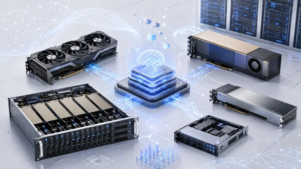
When this guide was first developed, the RTX 6000 Ada, A100 and H100 were prominent options for deep learning infrastructure. H200 and Blackwell have since expanded the choices. The decision principle has stayed the same: a newer or more powerful GPU is worthwhile only if the intended workload can use what it offers.
Buying a high-end accelerator without evaluating the application creates three common problems:
- The GPU and its required server platform can cost far more than the useful performance justifies.
- Small or poorly parallelized tasks may leave much of the compute capacity idle.
- Software designed for a single GPU may need substantial changes before it benefits from a multi-GPU system.
For a budget-constrained development team, an inference service or a shared research facility, consumer and workstation cards therefore belong on the shortlist alongside data center accelerators. The question is how much usable capacity the complete investment buys.
What historical benchmarks can teach us
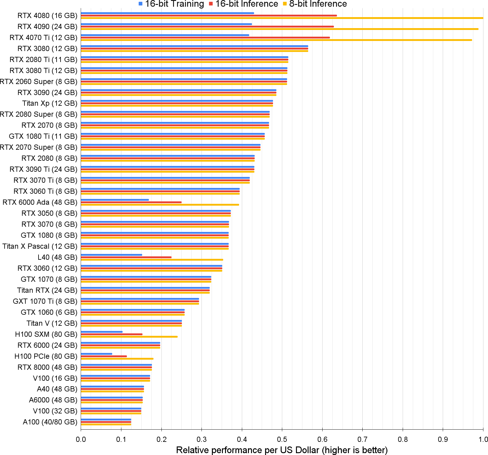
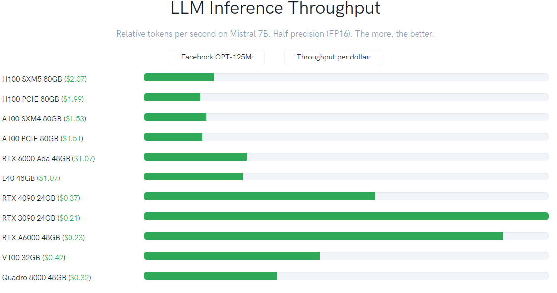
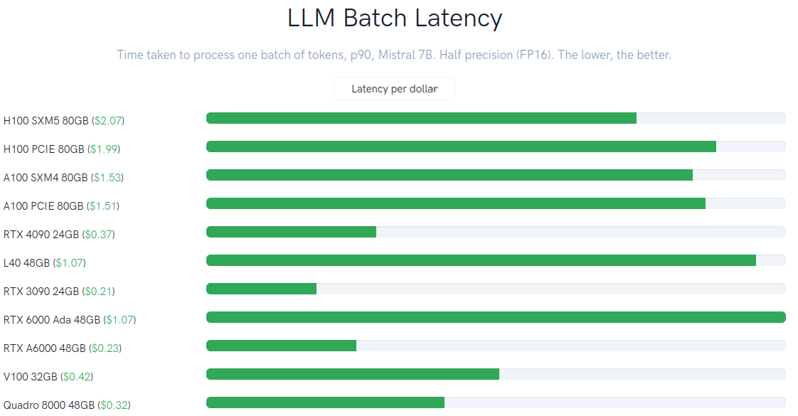
The chart below comes from Tim Dettmers’ 2023 analysis of GPUs for deep learning. In the workloads and prices considered there, cards such as the RTX 4090 offered attractive performance per cost relative to the A100. Those results illustrate a comparison method; they are not current prices or a ranking for every model.
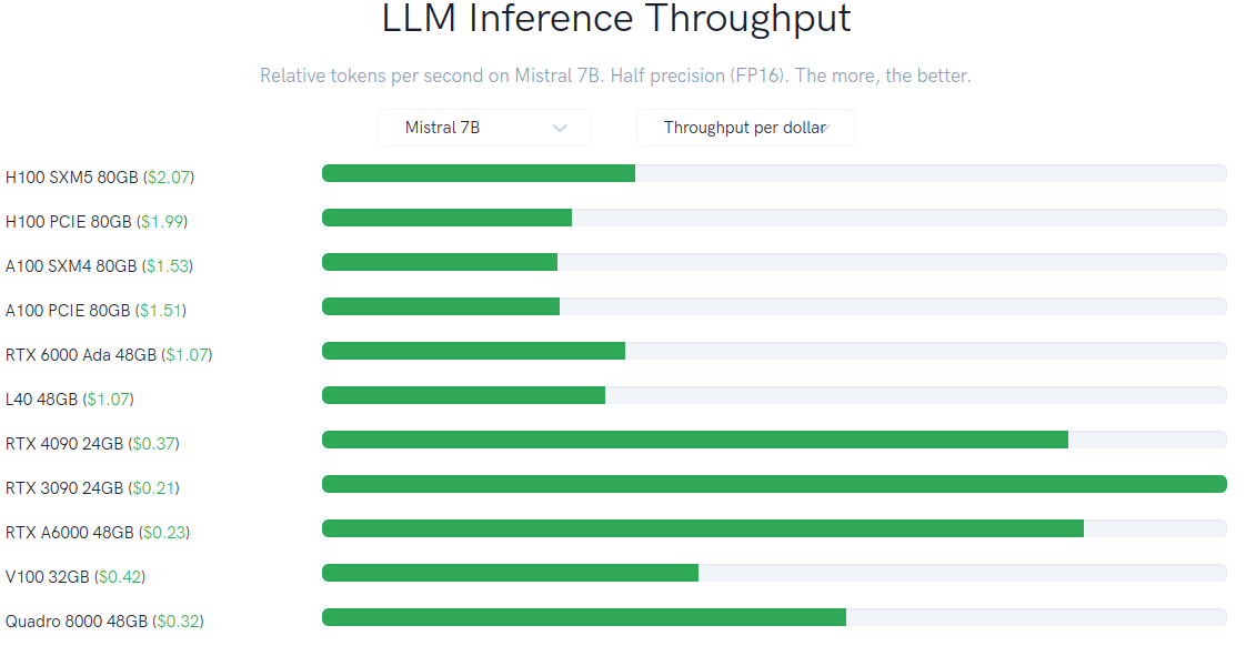
The following snapshots from TensorDock’s benchmarks show the same point for particular language-model workloads. Lower-cost cards can compare favorably in one test, while another workload changes the order. These are snapshots retained from the original article: rental prices, drivers and execution engines have changed since they were captured.
Training and inference place different demands on the hardware. In inference, the questions often concern whether the weights and KV cache fit, how many requests can run concurrently and how quickly each user receives an answer. Training also needs gradients, activations and optimizer state. Distributed training adds recurring communication between GPUs.
An inference result cannot therefore be carried over to training. Even within either category, model size, batch size, numerical precision and available memory can change the result. The distinction between a format listed on a specification sheet and the format actually used by the runtime is covered in INT8 or FP8: real GPU support.
Compare the complete deployment
NVIDIA supplies some consumer cards as reference designs, while board partners such as ASUS, MSI and Gigabyte offer their own versions. Their prices reflect more than the processor: cooler design, dimensions, power delivery, noise and other features can differ. A feature useful in a desktop gaming system may have little value in a machine dedicated to AI.
Build quality, price and integration requirements deserve more attention than decorative features. Many RTX 4090 variants are too large, or use an unsuitable airflow pattern, for dense server deployment. A compact or blower-cooled card must still be checked by its exact part number. A descriptive reseller name is not a substitute for an official specification or an OEM-supported configuration. See PCIe GPU server selection for the mechanical, thermal and electrical checks.
The cost comparison should include the host server, cooling and power provision, software preparation and expected utilization. A cheap GPU that requires extensive integration work may not be cheap to operate. Conversely, a costly integrated system may add little value if each job runs independently on one card.
A small, deliberate hardware portfolio
A shared compute service does not necessarily need one uniform GPU model for every customer. A limited set of configurations can serve different memory and performance requirements while keeping operations manageable. Standardize where it reduces support work, and introduce another card type when a distinct workload justifies it.
Performance-per-cost comparisons have a long history. For example, Lambda’s comparison of the RTX 2080 Ti, V100 and contemporary GPUs divided throughput by total system cost. Its numbers are historical, but the method remains useful.
For a purchase today, run the intended model with its actual input lengths, batch sizes and service targets. Compare the cost of the capacity that passes those tests. The strongest card on paper may be the right choice, but it should earn that position through the workload rather than its product name.
INT8 or FP8: what your GPU can actually run
An eight-bit model format does not define its execution path. Examine kernels, memory and output quality before choosing hardware for language-model inference.
GPU selection often starts with memory capacity and peak compute performance. If the model’s weights fit and its numerical format appears on the specification sheet, compatibility can look settled. Moving an INT8 model to a newer GPU can expose the weakness in that assumption: the model may fail at execution time or perform very differently from expectations.
The GPU selection guide uses workload fit and operating cost as the main decision criteria. This article examines one detail behind that decision: whether the software actually uses the capability being purchased. The focus is language-model inference. Training and other integer-compute workloads require their own evaluation.
INT8 and FP8 describe different numbers
INT8 and FP8 both use eight bits for the base representation of each value, but they do not encode that value in the same way. In common INT8 quantization schemes, an integer and a scale approximate a real number. Reconstructed values within a group sharing a scale are evenly spaced. FP8 assigns some bits to an exponent, so the spacing changes with magnitude. FP8 also typically needs scaling, as described in the TensorRT quantization documentation.
FP8 itself has multiple representations. E4M3 uses four exponent bits and three mantissa bits; E5M2 uses five and two, trading precision for a wider range. NVIDIA’s Transformer Engine primer explains the distinction. Floating-point representation alone does not guarantee a smaller error for a particular model.
In quantized-model names, W refers to weights and A to activations—the intermediate values passed through the layers. W8A8 specifies the bit widths of those two groups. It does not, on its own, identify integer or floating-point computation.
| Model description | Meaning | What still needs checking |
|---|---|---|
| INT8 W8A8 | Weights and activations in the quantized operations use eight-bit integers | Scaling, kernel support and excluded layers |
| FP8 W8A8 | Weights and activations in the quantized operations use eight-bit floating point | FP8 variant, scale format and operation coverage |
| W8A16 with INT8 weights | Weights are compressed; activations use sixteen bits | Weight reconstruction and the actual matrix-multiplication precision |
| FP8 KV cache | Attention keys and values are quantized | Weight formats and layer computation are configured separately |
These distinctions also appear in the vLLM quantization documentation. Accumulation precision is another independent choice: INT8 inputs, for example, can use INT32 accumulation. “An eight-bit model” does not describe every operation in the model.
Weight memory is only part of the requirement
Exactly 70 billion parameters stored at one byte each occupy 70 decimal GB, or about 65.2 GiB. That raw figure is the same for INT8 and FP8. It excludes scales, higher-precision layers, temporary buffers and runtime memory.
The KV cache also grows with context length and active requests. As the vLLM KV-cache guide explains, its format is configured separately. Quantizing the weights to eight bits does not automatically quantize the cache.
Measure memory at the required input length, output length and concurrency. Successfully loading a model does not establish the capacity to serve it. This extends the GPU product-family comparison: additional memory may make deployment possible, but service capacity depends on the whole working set.
The INT8/FP8 balance changes on B300
The difference between B200 and B300 is a useful example. The following figures are nominal dense rates per GPU. B200 and B300 use Table 3 on page 25 of NVIDIA’s Blackwell Architecture Technical Brief. The H200 SXM figures are obtained by removing the sparsity multiplier from the vendor’s published rates.
| GPU and reference configuration | Dense FP8, TFLOPS | Dense INT8, TOPS | Nominal FP8/INT8 rate ratio |
|---|---|---|---|
| H200 SXM | 1,979 | 1,979 | 1:1 |
| B200 in HGX | 4,500 | 4,500 | 1:1 |
| B300 in HGX | 4,500 | 150 | Approximately 30:1 |
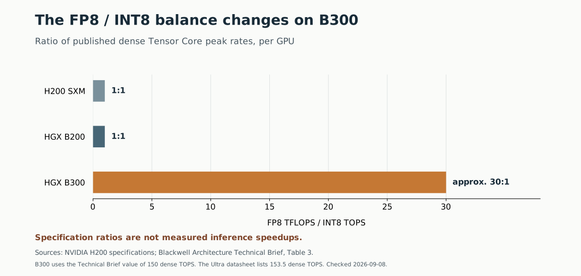
The Blackwell Ultra datasheet, page 5, lists 307 sparse INT8 TOPS for HGX B300, equivalent to 153.5 dense TOPS. The technical brief uses the rounded value of 150, which is the basis of this chart. Do not mix these figures with the GB300 NVL72 column or other configurations. The DGX/HGX comparison explains why platform distinctions matter.
There is also a difference between those documents and the live HGX product table, checked on 9 September 2026. The latter lists 3 sparse INT8 POPS for an eight-GPU HGX B300, equivalent to 187.5 dense TOPS per GPU. That is the basis used by the interactive comparison in this collection; against 4,500 dense FP8 TFLOPS, its ratio is 24:1. The chart above deliberately retains the technical brief’s 150-TOPS basis. These published figures are not identical, so preserve the source and configuration with every comparison and confirm the applicable specification for a purchase.
The reduction in nominal INT8 rate in this example occurs between B200 and B300; it does not apply to every Blackwell product. TFLOPS and TOPS also describe different types of operations here. Their ratio does not mean that an INT8 model will run thirty times more slowly.
From the specification sheet to an executable kernel
A kernel in this discussion is a compute function running on the GPU, such as a layer’s matrix multiplication—not the operating-system kernel. Three things must line up: the instruction must be valid for the target architecture, the library must provide a suitable implementation, and the execution engine must select it for the model.
Version 2 of the August 2026 preprint Spec Sheets Are Not Kernels audits that chain for Blackwell Ultra. It examines documentation and code at specified versions; it does not report speed or model-quality benchmarks. Its findings must be read within that scope.
| Layer | Finding in the case study | Limit of the conclusion |
|---|---|---|
| GPU instruction | PTX 9.3 lists tcgen05.mma with .kind::i8 for sm_100a, but not sm_103a | The absence of this fifth-generation path does not remove every INT8 capability |
| CUTLASS | At commit dcf215a, the generator excludes INT8 UMMA generation for target 103a | SM100 behavior cannot simply be assumed for SM103 |
| vLLM | The SM100 W8A8 path at commit 6c95a641 has no INT8 implementation | Even B200’s hardware capability is not necessarily used through this path |
| SGLang | The INT8 kernel examined at commit b20c375 covers architecture paths through Hopper | The finding concerns that kernel, not every INT8 method in SGLang |
The direct references are the PTX instruction manual, CUTLASS generator, vLLM operation-selection code and SGLang kernel. The code links deliberately pin commits. Check the installed version separately.
In the vLLM case, an initial compatibility check can pass before the missing compute path is exposed by the model’s first execution. A compatibility test must therefore continue at least as far as producing output. A smaller model using the same quantization method may expose the problem sooner, but final acceptance still requires the intended model: matrix shapes and model architecture can change kernel selection.
The study also discusses disabling a CUTLASS kernel with VLLM_DISABLED_KERNELS and examining a Triton fallback. That mechanism was tested on Ada, without a measured B300 performance result. The presence of a fallback is not sufficient evidence to recommend it for a B300 deployment.
Record the driver, libraries and execution-engine versions alongside the test results. The maintenance and security implications of this dependency chain are discussed in AI infrastructure security starts with the kernel and GPU.
Peak rates do not determine response time
Execution time depends on memory traffic, matrix dimensions, parallelism and implementation quality. NVIDIA’s matrix-multiplication performance guide describes how the ratio of operations to transferred data helps determine whether an operation is compute-bound or memory-bound.
Language-model prefill and token-by-token decode have different execution patterns. Increasing concurrency can improve compute utilization, but it also changes memory use and queuing delay. When FP8 and INT8 use different implementations, the benchmark compares complete configurations; the entire difference cannot be attributed to the numerical format.
Multi-GPU execution adds communication costs. Evaluate PCIe and SXM connectivity alongside precision. A higher arithmetic peak cannot compensate for a bottleneck elsewhere in the execution path.
Changing format requires a quality evaluation
If FP8 has a better-supported path on the target hardware, a migration is worth testing. Reinterpreting INT8 bytes as FP8 is not a valid model conversion. The numerical mapping and scales differ. When higher-precision weights are available, preparing the target quantization from those weights avoids adding another conversion on top of an already quantized representation.
Quality depends on the preparation method. SmoothQuant, for example, handles activation outliers to enable W8A8 with little degradation in its reported evaluations. A 2025 ACL study of quantization quality and efficiency examines several formats in the Llama-3.1 family under different deployment conditions. Neither result guarantees quality for a particular organization’s documents, language mix or specialized terminology.
Use test data that reflects the work: extracting amounts and names, preserving negation and conditions, producing evidence-based answers and returning structured output. A harmless change in wording is not equivalent to omitting a contractual condition or changing a monetary amount. Compare the quantized model with the baseline in a way that distinguishes those errors. For multilingual or domain-specific services, include the scripts, terminology and document structures that users actually submit.
Ask for a reproducible service test
A purchasing request should name an executable configuration: model version, quantization method, runtime, GPU and workload. The following information makes competing proposals meaningfully comparable.
| Area | What the test report should record |
|---|---|
| Model and environment | Weight version or hash, quantization method, GPU model, driver and runtime versions |
| Actual execution | Output from the intended model and the selected kernels for dominant operations |
| Capacity | Memory use at the target input length, output length and concurrency |
| Quality | Application-relevant errors against the baseline on representative data |
| Responsiveness | Time to first token, subsequent-token timing and latency percentiles |
| Cost | Usable serving capacity, model conversion and configuration maintenance |
The vLLM discussion of serving metrics distinguishes raw output rate from goodput: capacity that meets service targets. For an interactive application, the number of requests served within acceptable quality and latency limits is more useful than the largest token rate in an isolated run. Report loading and warm-up time separately from steady-state measurements.
If an existing INT8 deployment meets the service’s needs, the release of another GPU generation is not, by itself, a reason to migrate. For a new deployment, include model preparation, quality testing and software maintenance in the purchase comparison. A more expensive GPU with a mature FP8 path may cost less to operate, or retaining the current infrastructure may be the better choice. The same model and service test should decide between them.
Sources and numerical basis
Sources are linked beside the claims they support. The chart uses H200 specifications and Table 3 of the Blackwell technical brief; its downloadable data records the basis for each row. The source article’s numerical review date is 8 September 2026.
The software findings refer to the versions examined in the August 2026 study. This article does not report an independent B300 benchmark, and the underlying study did not audit TensorRT-LLM. The TensorRT reference near the beginning explains numerical formats only.
Why the fastest GPU does not necessarily deliver the fastest response
More compute and a higher token rate do not always mean a faster response. This article examines time to first token versus completion time, memory and concurrency, the division of work between GPUs and LPUs, and communication costs—so infrastructure choices reflect the capacity to serve requests at the required quality and latency.
From time to first token to token generation speed: how memory, concurrency and communication shape real inference performance
An inference system can produce more tokens per second while making the user wait longer for a response. It may even start writing sooner and finish later. These differences are not contradictions; they come from measuring different things under the shared label of “speed.”
The previous article, “INT8 or FP8: what your GPU can actually run”, examined why the performance listed in hardware specifications is not necessarily available in a model’s actual execution path. Here we go a step further: even when a model uses the right kernel and hardware acceleration, the card’s compute performance still cannot predict a service’s response time.
Infrastructure selection requires knowing which time must be reduced, how many concurrent requests must meet that target, and what achieving it will cost. This article, the second in this sequence within the GPU selection and AI infrastructure collection, examines that relationship.
When we say “fast,” what are we measuring?
A user sends a request, waits, sees the first part of the response, and then receives the rest. That experience involves at least two distinct timing measures: the wait before the response starts and the intervals at which subsequent parts are produced.
| Metric | Operational definition | Purpose |
|---|---|---|
| TTFT: time to first token | Time from sending the request to receiving the first content token | Measure the initial wait |
| TPOT: time per output token | Average time to produce tokens after the first token | Measure the pace of the continuing response |
| ITL: inter-token latency | Intervals between arrivals in the output stream, accounting for the number of tokens per chunk | Detect pauses and variability |
| Per-user token rate | Number of tokens after the first, divided by the time taken to receive them | Measure generation speed for one request |
| Aggregate output throughput | Total output tokens during the measurement interval, divided by its duration | Measure total service capacity |
| End-to-end latency | Time from sending the request to receiving the last token | Measure response completion time |
This distinction is consistent with inference benchmarking tools, but each tool’s precise definitions should accompany the results. Some tools measure the interval between response chunks, and each chunk may contain several tokens. GenAI-Perf metric documentation
In this article, let be the request submission time, the arrival of the first token, the arrival of the last token, and the number of output tokens:
For this request and this measurement convention, the per-user generation rate is therefore the reciprocal of TPOT. However, the reciprocal of the mean TPOT across several requests is not necessarily equal to their mean generation rate.
Client-side TTFT is not just GPU execution time: it also includes queuing, networking and request processing. In reasoning models, the first reasoning token may arrive much earlier than the first part of the final answer. AIPerf provides a separate “time to first non-reasoning output token” metric for this distinction. AIPerf metric definitions
Consequently, “a response in half a second” is incomplete without specifying where the measurement ends.
Starting sooner does not guarantee finishing sooner
Consider two hypothetical configurations:
| Configuration | TTFT | TPOT | Generation rate after the first token | Completion of a 101-token response | Completion of a 1,001-token response |
|---|---|---|---|---|---|
| A | 0.4 s | 40 ms | 25 tokens/s | 4.4 s | 40.4 s |
| B | 1 s | 20 ms | 50 tokens/s | 3 s | 21 s |
These figures are illustrative and do not represent specific hardware. They assume equal output lengths and that the stated TPOT values hold at both lengths. Completion time is calculated as:
Configuration A starts sooner; configuration B finishes long responses sooner. In this example, both finish a 31-token output at the same time; beyond that, B takes the lead.
This distinction matters when defining requirements. For a short answer, the initial wait may be the main concern. For report generation or a chain of dependent calls, completion time becomes more important. In an agentic system, the number of steps, the output length of each step and tool execution times must also remain in the calculation. Faster token generation does not shorten every part of the process.
Inference is not a uniform workload
In a typical autoregressive language model, prefill processes the input and stores the attention layers’ key and value information in the KV cache. Its output is also used to select the first token. Decode then continues generation using the previous state and extends the KV cache.
During prefill, many input tokens can participate in matrix computations. In conventional decode, each request advances by one token per step, so the opportunity to use compute units simultaneously differs. Small-batch decode can be sensitive to reading weights and the KV cache, whereas long prefill usually offers more opportunity to exploit compute capacity. This is a tendency: context length, model architecture, batch size and execution method can change the bottleneck. Transformer inference analysis in How To Scale Your Model
A good result for processing long inputs therefore does not necessarily mean faster generation for one user. A benchmark that reports only the combined total of input and output tokens may also show a larger number as input length increases, without making the continuing response any faster for the user.
Memory is more than a place to fit the model
Memory evaluation requires three separate questions: does the data fit, at what rate can it be read, and how long does it take to access the data needed?
More capacity can accommodate a model, a longer context or more active requests. Capacity alone, however, does not reduce the time needed to read the weights. Bandwidth describes a transfer rate and is not the same as access latency.
For an operation, an initial approximation is:
Here, is the number of computational operations, the compute rate, the volume of data exchanged with the memory level being examined, and that level’s bandwidth. The approximation assumes computation and transfer can overlap; execution overhead and insufficient parallelism can increase the time. NVIDIA’s guide to compute, memory and latency limitations
If data reads dominate the critical path, doubling matrix multiplication performance does not necessarily halve operation time.
For example, suppose a decode step must read exactly 70 GB of data from memory, with an effective bandwidth of 2 TB/s. Using decimal units, the lower bound for that read alone is 35 milliseconds:
This is not a speed prediction for a 70-billion-parameter model. It makes a specific assumption about the actual volume read in each step and does not separately account for attention, communication or overhead. Its value is to illustrate a limit that higher FLOPS alone cannot remove.
The KV cache must also be included in the memory budget. With conventional full-context attention, its requirements grow with sequence length and the number of active requests. Quantizing the cache or offloading it to host memory can reduce GPU memory use but has performance implications of its own; attention type and cache strategy also matter. Transformers guide to KV cache strategies
Fitting the weights does not demonstrate serving capacity.
Why can higher aggregate capacity slow down each user?
Running several requests in a batch can improve the use of weights and compute resources. Yet a system may aim to maximize aggregate output even if the interval between tokens increases for each request.
To clarify the difference, consider a steady, entirely hypothetical interval in which all requests are decoding:
| Case | Active decoding requests | Rate per request | Aggregate output rate |
|---|---|---|---|
| A | 20 | 80 tokens/s | 1,600 tokens/s |
| B | 100 | 30 tokens/s | 3,000 tokens/s |
Case B produces roughly 1.9 times as many tokens overall, but each user in case A receives output about 2.7 times faster. This table illustrates the arithmetic of a hypothetical situation, not a law describing how speed changes with concurrency.
In a real service, requests continually arrive and depart and have different lengths. Scheduling matters too. For example, vLLM documentation explains how chunked prefill divides long inputs into smaller pieces and schedules them alongside decode. Changing the scheduler’s token budget can alter the trade-off between TTFT and inter-token latency. vLLM optimization documentation
Two benchmarks using the same hardware and model but different scheduling policies can therefore produce different user experiences.
LPX: dividing the work even within decode
In the announced Vera Rubin architecture with Groq 3 LPX, NVIDIA assigns prefill and decode attention to the GPU, and decode FFN/MoE operations to the LPU. The entire decode phase is therefore not moved to the LPU. Intermediate data is exchanged between the two sides. NVIDIA’s architecture explanation
The diagram below is a conceptual reconstruction of that division of work. It omits subsidiary operations such as normalization, residual connections and tensor distribution details:
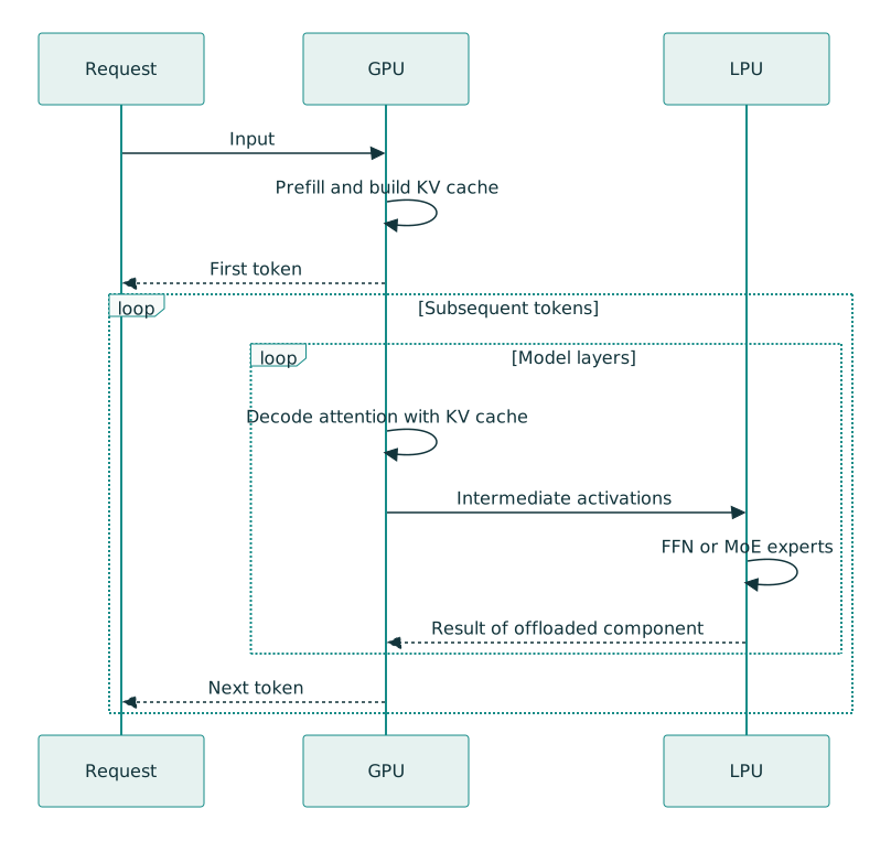
Download the diagram’s Mermaid source
This is different from separating prefill and decode into two processor groups. DistServe is an example of disaggregating the two phases to control interference and optimize serving under latency constraints; LPX extends the division to components within decode itself. Original DistServe paper
The reason to examine this example is architectural, rather than its product name: different parts of a request do not need the same proportions of memory capacity, bandwidth and compute performance.
Read memory figures at the correct scale
The official LPX page lists these specifications:
| Announced specification | Scale |
|---|---|
| 500 MB of SRAM | Per LPU |
| 150 TB/s of SRAM bandwidth | Per LPU |
| 256 LPU chips | One LPX rack |
| 128 GB of SRAM and 12 TB of DDR5 | One LPX rack |
| Approximately 40 PB/s of SRAM bandwidth | Aggregate across the rack |
| 640 TB/s of scale-up bandwidth | Rack level |
Source: Official NVIDIA Groq 3 LPX page
These are vendor-announced specifications. A rack’s aggregate SRAM bandwidth cannot be compared directly with the HBM bandwidth of a single GPU. DDR5 capacity is not SRAM capacity, either, and the intra-rack scale-up rate does not determine the usable rate of a particular GPU-to-LPU exchange.
Nor does a total of 128 GB of SRAM establish that all the weights of a very large model always fit in SRAM. Data placement, distribution and how often data moves must remain part of the analysis.
Communication determines the cost of dividing the work
Splitting an operation between two accelerators is beneficial when the execution savings exceed the additional transfer and coordination costs.
A transfer’s duration can be approximated as:
Here, is the fixed startup and delivery latency, the message size, and the path’s effective bandwidth. This simple model does not fully capture congestion or runtime variability, but it makes one distinction clear: for small messages, reducing fixed latency may matter more than increasing bandwidth.
For example, suppose a hypothetical design requires 80 dependent round trips to generate each token, and the total fixed cost of each round trip is 10 microseconds. The fixed communication contribution, before accounting for data volume, is 0.8 milliseconds. At 50 microseconds per round trip, it rises to 4 milliseconds.
This example is not an LPX specification. It shows why even small exchanges can matter in a frequently repeated loop.
Without overlap, a simple condition for offloading a component to be beneficial is:
In a real implementation, the relevant costs are those that remain on the critical path after overlap.
The same consideration applies to adding GPUs. Increasing tensor parallelism can free up more memory, but requires more coordination; vLLM documentation explicitly notes this overhead. vLLM parallelism considerations
Thus, “the model runs on four cards” does not mean “each user gets a response four times faster.”
What are the limits of a vendor’s claim?
For the combination of Vera Rubin NVL72 and LPX, NVIDIA claims up to 35 times more throughput per megawatt than GB200 NVL72 at approximately 400 tokens per second per user. This is a vendor claim about the configuration and scenario presented; it does not mean a 35-fold reduction in every request’s response time or universal LPX superiority. NVIDIA’s chart and explanation
Before using such a claim for procurement, the model, numerical precision, input and output lengths, concurrency, rack count, power measurement boundary and latency constraint must be known. A “tokens per megawatt” figure also does not by itself account for purchase price, networking costs, operations or actual capacity utilization.
Among the sources reviewed for this article, the LPX description rests on NVIDIA’s own documentation. Its figures are not presented here as independently reproduced results.
What capacity can actually be sold or used?
A service may achieve a high token rate in a benchmark while a substantial share of requests exceeds the permitted latency. That benchmark’s nominal capacity is not dependable serving capacity.
In our Targoman deployment under load (report in Persian), responses usually began in less than a second at low load; under pressure, the wait could reach the 20-second cutoff, at which point a request with no response started was cancelled. The system had roughly 300 concurrent requests during that incident, but not all completed successfully. This illustrates why usable capacity must count responses delivered within an acceptable time, rather than simply the requests present in the system.
Goodput addresses this issue by counting requests that meet specified constraints. In AIPerf, it is also distinct from the proportion of requests that comply with those constraints: a service rejecting many requests should not be judged successful simply because the remaining responses are fast. AIPerf goodput guide
For a particular service, an initial target might be: “At least 95% of requests must have both TTFT below two seconds and TPOT below 50 milliseconds.” These numbers are examples and should be derived from product requirements.
The emphasis on “both” is deliberate. Reporting the 95th percentile of each metric separately does not guarantee that the same 95% of requests meet both conditions.
Response quality also requires separate evaluation. Shortening the output or changing the model may improve timing, but a comparison remains valid only if the output still meets the application’s needs.
Define acceptance tests from service requirements
Before comparing cards, the test specification must be fixed and reproducible:
| Test area | What to record |
|---|---|
| Model and quality | Weight version, tokenizer, quantization and response acceptance criteria |
| Input and output | Length distributions, language, multi-turn context and actual output length |
| Incoming load | Arrival rate, concurrency, traffic bursts and test duration |
| Execution engine | Versions, batching, parallelism, chunked prefill and cache settings |
| Acceleration features | Whether prefix caching and speculative decoding are enabled |
| Latency | TTFT and TPOT distributions, streaming pauses and completion time |
| Capacity | Aggregate output rate, successful requests, errors, timeouts and goodput |
| Infrastructure and cost | Card and server counts, topology, power consumption and total configuration cost |
A single-user test helps establish a lower latency bound but does not determine service capacity. Increase the load and identify the point beyond which user experience constraints no longer hold. A fixed-concurrency test must also be distinguished from a fixed-arrival-rate test: in the former, a slower service can automatically delay the next request and reduce the pressure applied.
For Persian content, the sample must contain real Persian inputs. “Tokens per second” does not necessarily represent the same volume of text across two tokenizers, so comparing different models also requires assessing quality and the time taken to complete a common task.
The objective must also be explicit: isolate the hardware’s effect, or compare the best deployable service. For the former, settings should be as similar as possible. For the latter, each stack can be optimized, provided differences are documented and the quality criterion is preserved.
GPU selection starts with defining the response you need
When buying inference infrastructure, “Which card is faster?” is premature. First establish whether responses are short or long, how many concurrent requests are expected, what latency is acceptable, and which part of execution consumes the time.
LPX illustrates an architectural response to the different needs of inference components. Its existence does not imply that every service needs heterogeneous hardware. Sometimes better scheduling, the right software stack or reduced memory pressure solves the problem; sometimes dividing work between processors is worth the communication cost.
The purchasing criterion should be the capacity to serve requests at the required quality and latency. Compute, memory and networking are means to that end. Ranking higher in one of those columns alone does not establish better response performance.
Where does GPU confidential computing overhead come from?
Why does one confidential B200 inference stack lose 39% of throughput while another incurs only a few percent? A close reading of the measurements: command submission, PCIe, encrypted NVLink and the serving software.
From command submission and PCIe transfers to encrypted NVLink and the inference stack
Confidential computing aims to protect data, model weights and intermediate execution state even from the infrastructure administrator, host operating system and hypervisor. To assess its cost, we need to ask which parts of execution incur overhead, how much of each request is spent there, and how the software stack hides or amplifies that cost.
A recent preprint on confidential computing performance on NVIDIA B200 reports two apparently conflicting results: inference overhead of roughly 1–3% with a properly configured stack, and throughput losses of 30–40% in some unpatched configurations.
The article on actual INT8 and FP8 support showed why nominal format support does not guarantee that a workload uses it. The article on latency and throughput explained why the fastest GPU does not necessarily produce the fastest response. This third installment in that sequence within the GPU selection guide goes one layer deeper: even with the hardware and model held constant, the security architecture and inference software determine the cost of protecting the data.
What, exactly, becomes confidential?
In the tested system, an Intel TDX confidential VM protects CPU memory and state from the host, while NVIDIA Confidential Computing extends protection to the GPU.
The earlier discussion of infrastructure security from the kernel to the GPU examined access through lower layers of the system. Here we examine the cost of protecting those boundaries:
- VM memory and CPU state;
- host-memory-to-GPU transfers over PCIe;
- GPU memory;
- the command path from the host to the GPU management processor;
- communication between GPUs over NVLink;
- and the attestation chain for hardware, firmware and the execution environment.
In Intel TDX, the VM’s private memory is isolated from the virtual machine monitor, or VMM, and host software.
According to NVIDIA’s confidential computing guide, Blackwell also supports encrypted NVLink in multi-GPU mode. CPU–GPU transfers can use encrypted bounce buffers or, on compatible platforms, TDISP/IDE.
Enabling encryption therefore affects several boundaries, each with a different cost pattern.
Which system do these measurements describe?
This article analyzes version 2 of the preprint, published on 1 September 2026. The measurements below belong to the paper’s authors; they are not experiments conducted for this article.
| Component | Test configuration |
|---|---|
| Host | Dual-socket Intel Xeon 6767P server |
| GPUs | Eight NVIDIA B200 GPUs connected through NVLink |
| Confidential environment | Intel TDX with NVIDIA CC |
| Operating system | Ubuntu 24.04.3 |
| Guest driver | NVIDIA 595.71.05 Open Driver |
| Inference engines | SGLang 0.5.13.post1 and a patched branch; vLLM 0.21.0 and 0.22.0 |
| Models | Dense and MoE models using NVFP4, FP8, AWQ and bf16 |
| Comparison | Paired CC-on and CC-off runs on the same host, disk and GPUs |
Within each comparison, the hardware is held constant and TDX/CC is toggled. Framework versions, models and configurations differ across experiments, however. Comparisons within a row are more informative than treating unrelated rows as interchangeable.
The authors also report that clean measurements required a reboot. Residual GPU state produced an apparent 16% overhead in one run, whereas a clean run of the same workload showed about 2%. Leftover state can therefore create a difference much larger than the overhead being measured.
Compute is not the main bottleneck
The paper’s central finding is that matrix multiplication, GEMM and HBM access were not the main sources of overhead in this configuration. Most of the cost appeared at communication boundaries:
- host-to-GPU command submission;
- CPU–GPU transfers over PCIe;
- GPU–GPU communication over encrypted NVLink.
The arithmetic itself did not necessarily become slower. Delivering commands and data, and coordinating GPUs, became more expensive.
First cost: every small command has a fixed price
When the host launches a kernel, the command passes through a protected control path to the GPU System Processor, or GSP. The study measured roughly 12 additional microseconds per kernel submission on one GPU:
| Operation | CC off | CC on | Difference |
|---|---|---|---|
| Kernel submission | 3.45 µs | 15.7 µs | About 12 µs |
| Synchronization without submission | 1.62 µs | 1.67 µs | Almost zero |
Twelve microseconds becomes significant when a decoding step contains dozens or hundreds of separate submissions. In the paper’s microbenchmark, a step contained about 181 kernels. Eager execution submitted them again on every step:
| Execution mode | CC off | CC on | Time ratio |
|---|---|---|---|
| Eager | 2,644 µs per step | 6,358 µs | 2.41× |
| Full CUDA graph | 2,500 µs | 2,589 µs | 1.04× |
A CUDA graph records the operations in advance and replays a graph instead of submitting hundreds of individual commands. In this microbenchmark, that reduced a large control-path penalty to a few percent.
“CUDA graphs enabled” is not a sufficient description, though. A framework that splits the graph at every attention layer can still leave roughly 185 host submissions per step. The actual submission count matters more than the setting’s name.
A rough expression for this cost is:
The shorter the compute step and the more submissions it contains, the larger the contribution of that fixed cost.
Second cost: encrypted PCIe is about more than bandwidth
In this stack, host–GPU transfers use AES-GCM and driver-managed bounce buffers. Large transfers pay a cost roughly proportional to their byte count. Small transfers are more sensitive to cryptographic setup and call overhead.
In the paper’s tests:
- the transfer rate was 7.21 GB/s at 1 MB and roughly 9.4–9.6 GB/s at 16 and 64 MB;
- transfers of 64 KB or less were dominated more by a fixed overhead of about 3–6 µs;
- adding host threads did not improve encryption throughput for one GPU session.
This limitation is visible during initial weight loading. If weights and the KV cache remain on the GPU afterward, it need not recur in every token’s critical path.
The more damaging problem was reading the sampling result back from the GPU at the end of each decoding step. In the unpatched stack, a small device-to-host copy that should overlap the next step’s computation effectively became synchronous and stalled the scheduler. The GPU waited, utilization fell, and the throughput loss exceeded the time spent on AES computation itself.
That is where the 30–40% result emerges.
Why does one experiment show 39% and another less than 1%?
With released, unpatched SGLang, Qwen3-8B on one B200 with overlap enabled produced these results:
| Concurrency | Throughput without CC, tokens/s | Throughput with CC, tokens/s | Throughput loss |
|---|---|---|---|
| 16 | 3,828 | 2,513 | 34.4% |
| 32 | 6,931 | 4,534 | 34.6% |
| 64 | 11,137 | 6,805 | 38.9% |
At concurrency 64, time per output token rose from 5.48 to 8.28 ms, and time to first token from 259 to 409 ms. The “39%” refers to lost throughput; some latency measures increased by more than that.
The small D2H copy no longer hid behind computation. Scheduling became serialized, and GPU utilization fell from 74% to 57%.
After moving D2H copies to an asynchronous worker and applying CC-compatible fixes, a separate single-GPU experiment with Qwen2.5-72B-AWQ showed overhead between −0.2% and +0.6% across concurrency settings: effectively measurement noise. This was a different model, not a before-and-after comparison on the same model. Across ten input/output shapes, median overhead was 1.2% and the worst result was 6.5%.
The 30–40% loss is therefore not an inherent GPU encryption tax. It is an interaction between confidential mode and a specific unpatched stack. Near-zero overhead is also configuration-dependent: the framework, model and workload shape still matter.
Third cost: encrypted NVLink
Adding a second GPU introduces another path. Collective operations such as all-reduce and all-to-all must run over encrypted NVLink.
A microbenchmark on four B200 GPUs in one NUMA node reported:
| Metric | CC on, GB/s | CC off, GB/s | Calculated reduction |
|---|---|---|---|
| Copy Engine, one-way read | 8,070 | 9,170 | 12.0% |
| Copy Engine, one-way write | 8,278 | 9,292 | 10.9% |
| SM-based read | 7,693 | 9,388 | 18.1% |
| NCCL all-reduce | 156 | 185 | 15.7% |
| NCCL all-to-all | 130 | 149 | 12.8% |
The NCCL percentages are calculated from the values in each row; the original table’s “10%” labels do not match those values. The Copy Engine and SM rows are the reported D2D benchmark metrics, not a single NVLink connection’s bandwidth specification. Median latency for a small P2P write also increased from 3.7 to 14.5 µs, almost fourfold.
These results do not imply a 10–18% loss for the entire service. The end-to-end effect depends on the share of each step spent communicating between GPUs.
If a collective occupies only 20% of the critical path and encryption makes that part 10% slower, its direct contribution to total time is much smaller than 10%. A workload that is almost entirely communication-bound is more exposed to the raw communication penalty.
This is another reason the difference between PCIe and SXM is more than a mounting detail: the route and volume of GPU communication also affect confidential execution costs.
Two independent dimensions of overhead
| Cost dimension | Behavior | Ways to reduce it |
|---|---|---|
| Fixed host-operation cost | Repeats with submissions, synchronization and readbacks | More complete CUDA graphs, fewer graph splits, asynchronous D2H worker |
| NVLink traffic cost | Varies with encrypted inter-GPU traffic | Fewer unnecessary collectives and suitable parallelism |
Larger batches can spread fixed submission costs across more requests. They can also increase collective traffic. Batching may improve the first dimension while making the second more visible until it reaches a plateau. There is no single batch size that minimizes both costs for every workload.
Under which conditions was the 1–3% result obtained?
The principal multi-GPU result concerns MiniMax-M2.7, an MoE model with about 229 billion total parameters and 6 billion active parameters, on eight B200 GPUs.
At the reference point of 1,024 input tokens, 2,048 output tokens and concurrency 32:
- TP8 showed 2.8% and 3.6% overhead in two sets of five repeated runs;
- TP4 showed about 1.5% overhead;
- halving the tensor-parallel width to TP4 retained 94% of TP8 throughput.
“About 1–3%” describes a particular performance regime: a patched stack with piecewise CUDA graphs and overlap enabled, a decoding-heavy workload, and parallelism suited to the model. It is not a result for every workload or every configuration of the same server.
| Measured scenario | Reported overhead | Main mechanism |
|---|---|---|
| One GPU, overlap off | About 2% | Residual command-path cost |
| One GPU, overlap on, unpatched | 34–39% | Lost compute/copy overlap |
| One GPU, graphs and patched stack | Below 1% in the main sweep | Cost removed from the critical path |
| MoE with TP8 | About 2.8–3.6% | Encrypted all-reduce |
| MoE with TP4 | About 1.5% | Less NVLink traffic |
| Qwen3.5 with DP-attention and EP, 32,768-token input | About 2% | No attention all-reduce |
| Eight-GPU training | 11–24% longer steps | Frequent training collectives |
Inference rows measure throughput loss; training measures increased step duration. Their denominators are different. The training configurations also differ substantially:
| Training test on eight GPUs | Step time without CC | Step time with CC | Time increase |
|---|---|---|---|
| Dense bf16, TP8 | 13.95 s | 15.8 s | 13.3% |
| Dense delayed FP8, TP8 | 14.5 s | 18.0 s | 24.1% |
| Tuned MoE, EP8 | 2.16 s | 2.40 s | 11.1% |
These percentages are calculated from the reported step times. The FP8 experiment has the largest increase.
How does output length change the result?
In a MiniMax-M2.7 sweep with TP8, 1,024 input tokens and concurrency 32, longer outputs spread the encrypted prefill cost across more decoding steps:
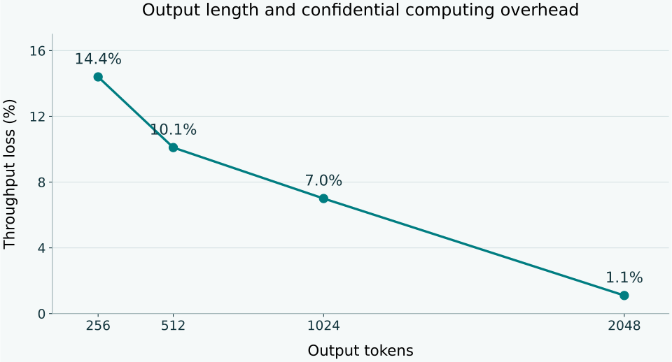
| Output tokens | Without CC, tokens/s | With CC, tokens/s | Throughput loss |
|---|---|---|---|
| 256 | 1,701.0 | 1,456.0 | 14.4% |
| 512 | 2,300.5 | 2,068.4 | 10.1% |
| 1,024 | 2,551.4 | 2,371.6 | 7.0% |
| 2,048 | 2,530.7 | 2,504.0 | 1.1% |
The chart uses the paper’s sweep values. Most points were single passes over random data, and the authors report variation of roughly two percentage points. Five-repeat measurements at the same 1,024-input/2,048-output shape yielded 2.8–3.6%, not 1.1%. The chart supports the direction of change more strongly than the final decimal place of each point.
In this experiment, prefill occupied a larger share of total execution time for short responses. Longer decoding reduced its relative contribution.
Longer context does not always reduce overhead
The effect depends on parallelism. In the MiniMax-M2.7 NVFP4 experiment on four GPUs with TP2/EP4/DP2, increasing input from 4,096 to 32,768 tokens raised overhead from 9% to 14.5%, associated with more prefill all-reduce traffic.
In the Qwen3.5-397B-A17B FP8 experiment on eight GPUs with DP8/EP8, attention did not require inter-GPU all-reduce. Over the same input range, overhead fell from 11.1% to 1.9%. More computation amortized fixed costs and expert communication.
These experiments differ in model, numerical format and GPU count, so the difference cannot be attributed solely to parallelism. Both used 256 output tokens and concurrency 32.
“Longer context reduces CC overhead” is therefore as incomplete as its opposite. The determining question is how much additional computation and how much additional encrypted communication the longer context creates.
More parallelism is not always better
Tensor parallelism exchanges parts of activations between GPUs at each layer, usually through all-reduce. In confidential mode, that traffic is encrypted. If the model runs adequately without eight-way TP, spreading it across more ranks can simply increase communication.
At the paper’s reference point, reducing TP8 to TP4 approximately halved CC overhead to 1.5% while preserving 94% of throughput.
The lesson is not simply to use fewer GPUs. GPU count and the width of a tensor-parallel group are different concepts. A larger deployment can still keep each replica or TP group only as wide as the model needs.
For MoE models, expert and data parallelism may also require less synchronous communication than tensor parallelism. The choice must still be tested with the actual model, batch size, context length and topology.
The software stack is part of the security architecture
The comparison of Ollama, vLLM, SGLang and llama.cpp starts with the service’s requirements. For confidential execution, the data-transfer behavior of a specific software version becomes another selection criterion. Framework decisions determine how often a small hardware cost recurs and where it enters the critical path.
The study identifies several influential changes:
- use CUDA graphs and reduce graph splitting;
- move token readback to a separate asynchronous worker;
- avoid requesting unsupported pinned host memory;
- use the global timer rather than CUDA events in the autotuner;
- choose fusions that do not depend on multicast blocked in CC mode;
- keep weights and the KV cache resident on the GPU;
- avoid weight streaming, CPU expert offload and KV offload on the critical path;
- size TP for the model rather than for the available GPU count.
An NVIDIA report published on 2 July 2026 also emphasizes an asynchronous D2H worker, CC-compatible timing and piecewise CUDA graphs. Its HGX B300/Qwen3.5 tests report roughly 1–8% impact across workload shapes. Those numbers cannot replace or be pooled with the B200 measurements, but they also show the importance of the stack’s version and configuration.
What did the study not measure?
Startup and attestation
The study did not measure confidential VM creation, GPU initialization, secure-session establishment, CPU/GPU attestation or key delivery.
Attestation usually precedes the release of secrets and workload execution rather than recurring for every inference request. Startup time may still matter for short-lived workloads, aggressive autoscaling or serverless services. This study supplies no measurement for it.
Communication between hosts
All results come from one physical host. RDMA, multi-server GPU communication, prefill/decode disaggregation and inter-node KV-cache transfer were not benchmarked.
The paper explains that CC restricts GPUDirect RDMA and conventional pinned buffers in the tested stack. Transfers may have to follow a GPU–CPU–CPU–GPU path. That is an architectural issue, not a quantitative benchmark for multi-node clusters.
Security assurance
The study neither audited nor proved a security property. Resistance to a specified attacker, firmware security, supply chains, key management, attestation policy and side-channel coverage were outside the tests.
Administrator powers, logging and information recoverable from outputs still require a separate examination of indirect data access.
Other hardware
The results concern B200, Intel TDX and specific driver/framework versions. They cannot be directly transferred to H100, B300, other GPUs, AMD SEV-SNP, TDISP/IDE platforms or later software generations.
What should an acceptance test record?
A procurement or acceptance test should capture at least the following:
| Area | Required details |
|---|---|
| Hardware | CPU/GPU models, GPU count, NUMA and NVLink topology |
| Security | TEE type, CC mode, firmware version, attestation method |
| Software | Driver, CUDA, NCCL, framework and CC patch versions |
| Model | Weight version, precision, dense or MoE architecture |
| Workload | Input/output-length distributions, batch size, arrival rate |
| Parallelism | TP, PP, DP and EP, with each group’s width |
| Scheduling | CUDA graphs, piecewise graphs, overlap, chunked prefill |
| Memory | Weight/KV-cache location and offload settings |
| Results | TTFT, TPOT, throughput, goodput, errors, utilization |
| Lifecycle | Startup, attestation and key-delivery time where relevant |
| Scale | Single or multiple hosts and actual communication paths |
Run the same workload with and without CC on identical hardware and data. Repeat each point and report dispersion alongside the mean or median. A one- or two-percent difference in a single run may be no more than measurement noise.
Before choosing a configuration
If throughput loss rises from 34% to 39% as concurrency increases while GPU utilization falls, first investigate result readback and scheduling. If the loss grows with input length and collective traffic, TP width and inter-GPU communication become more relevant. These conditions call for different fixes.
In the paper’s reference configuration, TP4 retained about 94% of TP8 throughput with less confidentiality overhead. That comparison is more useful than a universal “CC tax”: which configuration serves the actual workload at the required latency and capacity?
GPU server reference
Define the card, then choose the server
This table distinguishes PCIe add-in cards from integrated HGX/SXM/OAM systems. Compare interface generation, card count and width, power, cooling, rack height and depth together. Every record links to a manufacturer product page or technical guide.
Data last reviewed8 September 2026
What qualification means hereManufacturer qualification is shown only when the exact GPU model is named on the server's official product page, QuickSpecs or QPL. Matching dimensions and power without explicit card qualification is marked as requiring BOM confirmation.
Selection and compatibility filters 22 Results
Results22of 32 reference models
PCIe card systems22After the current filters
Explicit card qualification—Select My GPU first
Selected for comparison0Up to 4 servers
| Compare | Details | ||||||||||
|---|---|---|---|---|---|---|---|---|---|---|---|
 ASRock Rack4U10G-ROME2/2TPrevious generation ASRock Rack4U10G-ROME2/2TPrevious generation | PCIe add-in cards | Previous generation | PCIe Gen4 | 10 dual-slot · 20 single-slot | 4U | Direct to CPU | Passive | BOM required | Check the exact model in the configurator/QPL | ||
 DellPowerEdge XE7745Current generation DellPowerEdge XE7745Current generation | PCIe add-in cards | Current generation | PCIe Gen5 | 8 dual-slot · 16 single-slot | 4U | Through a PCIe switch | Passive | 600 W | NVIDIA H200 NVL PCIe, NVIDIA RTX PRO 6000 Blackwell Server Edition | ||
 GIGABYTEG495-DB1-AM1Announced GIGABYTEG495-DB1-AM1Announced | PCIe add-in cards | Announced | PCIe Gen6 | 10 dual-slot | 4U | Through a PCIe switch | Passive | BOM required | Check the exact model in the configurator/QPL | ||
 SupermicroGPU A+ Server AS-4125GS-TNRT2Current generation SupermicroGPU A+ Server AS-4125GS-TNRT2Current generation | PCIe add-in cards | Current generation | PCIe Gen5 | 10 dual-slot · 10 single-slot | 4U | Through a PCIe switch | Passive / Active | BOM required | NVIDIA H200 NVL PCIe, NVIDIA H100 PCIe, NVIDIA L40S, NVIDIA RTX PRO 6000 Blackwell Server Edition | ||
| SupermicroGPU SuperServer SYS-420GP-TNRPrevious generation | PCIe add-in cards | Previous generation | PCIe Gen4 | 10 dual-slot · 10 single-slot | 4U · 737 mm | Through a PCIe switch | Passive / Active | BOM required | NVIDIA H100 PCIe, NVIDIA A100 PCIe, NVIDIA A40, NVIDIA A10, NVIDIA L40S, NVIDIA RTX A6000 | ||
 HPEProLiant Compute DL380a Gen12Current generation HPEProLiant Compute DL380a Gen12Current generation | PCIe add-in cards | Current generation | PCIe Gen5 | 10 dual-slot | 4U | Through a PCIe switch | Passive | 600 W | NVIDIA H200 NVL PCIe, NVIDIA H100 NVL PCIe, NVIDIA RTX PRO 6000 Blackwell Server Edition, NVIDIA L40S, NVIDIA L4 | ||
| HPEProLiant DL380a Gen11Current generation | PCIe add-in cards | Current generation | PCIe Gen5 | 4 dual-slot · 8 single-slot | 2U · 816 mm | Direct to CPU | Passive / Active | BOM required | NVIDIA L40S, NVIDIA L4, NVIDIA A10, NVIDIA RTX 6000 Ada | ||
 LenovoThinkSystem SR655 V3Current generation LenovoThinkSystem SR655 V3Current generation | PCIe add-in cards | Current generation | PCIe Gen5 | 3 dual-slot · 8 single-slot | 2U | Direct to CPU | Passive / Active | BOM required | NVIDIA L40S, NVIDIA L4, NVIDIA A10, NVIDIA RTX 6000 Ada | ||
| LenovoThinkSystem SR675 V3Current generation | PCIe add-in cards | Current generation | PCIe Gen5 | 8 dual-slot · 8 single-slot | 3U · 892 mm | Through a PCIe switch | Passive / Active | 600 W | NVIDIA H200 NVL PCIe, NVIDIA RTX PRO 6000 Blackwell Server Edition, NVIDIA L40S | ||
| ASRock Rack4U8G-EGS2Current generation | PCIe add-in cards | Current generation | PCIe Gen5 | 8 dual-slot | 4U | Direct to CPU | Passive | BOM required | Check the exact model in the configurator/QPL | ||
 ASUSESC8000A-E11Previous generation ASUSESC8000A-E11Previous generation | PCIe add-in cards | Previous generation | PCIe Gen4 | 8 dual-slot · 8 single-slot | 4U | Direct to CPU | Passive / Active | BOM required | NVIDIA A100 PCIe, NVIDIA A40, NVIDIA A10, NVIDIA RTX A6000 | ||
| ASUSESC8000A-E12Current generation | PCIe add-in cards | Current generation | PCIe Gen5 | 8 dual-slot · 8 single-slot | 4U | Direct to CPU | Passive / Active | BOM required | NVIDIA H100 PCIe, NVIDIA L40S | ||
| ASUSESC8000A-E13Current generation | PCIe add-in cards | Current generation | PCIe Gen5 | 8 dual-slot · 8 single-slot | 4U | Direct to CPU | Passive / Active | 600 W | NVIDIA H200 NVL PCIe, NVIDIA RTX PRO 6000 Blackwell Server Edition, NVIDIA RTX PRO 4500 Blackwell Server Edition | ||
| GIGABYTEG492-H80Previous generation | PCIe add-in cards | Previous generation | PCIe Gen4 | 8 dual-slot · 8 single-slot | 4U | Direct to CPU | Passive | BOM required | NVIDIA A100 PCIe, NVIDIA A40, NVIDIA A10 | ||
| GIGABYTEG494-SB0-AAP2Current generation | PCIe add-in cards | Current generation | PCIe Gen5 | 8 dual-slot · 8 single-slot | 4U | Through a PCIe switch | Passive | 600 W | NVIDIA H200 NVL PCIe, NVIDIA RTX PRO 6000 Blackwell Server Edition | ||
| GIGABYTEG494-ZB4-AAP2Current generation | PCIe add-in cards | Current generation | PCIe Gen5 | 8 dual-slot · 8 single-slot | 4U | Through a PCIe switch | Passive | 600 W | NVIDIA H200 NVL PCIe, NVIDIA RTX PRO 6000 Blackwell Server Edition | ||
| SupermicroGPU SuperServer SYS-421GE-TNRT3Current generation | PCIe add-in cards | Current generation | PCIe Gen5 | 8 dual-slot · 8 single-slot | 4U | Through a PCIe switch | Passive / Active | BOM required | NVIDIA H200 NVL PCIe, NVIDIA H100 NVL PCIe, NVIDIA H100 PCIe, NVIDIA L40S, NVIDIA L4, NVIDIA RTX 6000 Ada | ||
| SupermicroGPU SuperServer SYS-422GA-NRTCurrent generation | PCIe add-in cards | Current generation | PCIe Gen5 | 8 dual-slot · 8 single-slot | 4U · 737 mm | Through a PCIe switch | Passive / Active | 600 W | NVIDIA RTX PRO 6000 Blackwell Server Edition | ||
| DellPowerEdge XE7740Current generation | PCIe add-in cards | Current generation | PCIe Gen5 | 8 dual-slot · 8 single-slot | 4U · 886.7 mm | Through a PCIe switch | Passive | 600 W | NVIDIA H200 NVL PCIe, NVIDIA H100 NVL PCIe, NVIDIA RTX PRO 6000 Blackwell Server Edition, NVIDIA L40S, NVIDIA L4 | ||
 FujitsuPRIMERGY GX2550 M8sCurrent generation FujitsuPRIMERGY GX2550 M8sCurrent generation | PCIe add-in cards | Current generation | PCIe Gen5 | 8 dual-slot | 4U | Through a PCIe switch | Passive | 600 W | NVIDIA H200 NVL PCIe, NVIDIA RTX PRO 6000 Blackwell Server Edition | ||
| HPEProLiant Compute DL345 Gen12Current generation | PCIe add-in cards | Current generation | PCIe Gen5 | 4 dual-slot | 2U | Direct to CPU | Passive | BOM required | NVIDIA RTX PRO 4500 Blackwell Server Edition, NVIDIA L40S, NVIDIA L4 | ||
| SupermicroSuperWorkstation SYS-532AW-CCurrent generation | PCIe add-in cards | Current generation | PCIe Gen5 | 1 dual-slot · 1 single-slot · 1 triple-slot | 4U | Direct to CPU | Active | 575 W | GeForce RTX 5090 |
PCIe backward compatibility does not preserve link speed
A Gen4 card runs at Gen4 in a Gen5 slot. A Gen5 card may negotiate down to Gen4, but the table excludes that by default to avoid accepting a potential bandwidth bottleneck.
Chassis capacity is not installation approval
Eight dual-slot positions describe the basic layout. Card power, active/passive cooling, ambient temperature, cabling and the QPL may reduce the supported count.
Exact OEM part numbers matter
A matching GPU model name is not enough in an enterprise server: the general-market card may differ from the version carrying the server manufacturer's part number or FRU code.
Beyond the GPU: CPU, memory, storage and networking
Size the rest of a GPU server around data preparation, memory use, storage traffic and the application's communication pattern.
A multi-GPU server can accelerate one parallel job or run several independent jobs at once. The second use is valuable even when the application cannot distribute a single task across GPUs: users can share the chassis, power provision and rack space. In both cases, the host platform must supply data and services fast enough to make the GPUs useful.
This article covers CPU, system memory, storage and networking. For the physical installation of particular cards, use the PCIe server selection guide.
CPU capacity and topology
Although GPUs perform much of the computation in many AI workloads, CPUs still prepare data, schedule work and collect results. Tokenization, decoding, augmentation and parts of a retrieval pipeline may consume significant CPU time. Work that does not need a GPU can sometimes run on conventional servers, keeping scarce accelerator capacity available for the tasks that benefit from it.
There is no universal CPU brand or minimum clock speed for a GPU server. In a multi-GPU configuration, the number of PCIe lanes, the attachment of slots to each CPU, memory channels and bandwidth can matter more than nominal core count. The processor must also be supported in the selected chassis configuration.
NUMA topology deserves particular attention in a dual-socket server. A GPU, its data-loading process and its network adapter may not all be attached to the same CPU. The resulting traffic paths can affect performance even when the headline specifications appear sufficient. Evaluate the proposed topology with the application, rather than treating the CPU as an isolated purchase.
System memory
RAM requirements depend on how the application uses the host. A well-optimized inference workload may keep the model and active working set on the GPU and need relatively little host memory. Data loaders, caches, preprocessing, CPU offload and concurrent users can change that requirement considerably.
A fixed ratio between system RAM and total GPU memory is only a rough planning shortcut. It does not replace measurement. The amount of data retained in memory, the number of workers and the application’s allocation behavior are more useful inputs.
In one deployment I examined, a team used more than a terabyte of host memory and concluded that the server needed an upgrade. Debugging reduced the requirement to roughly 64 GB. That observation is not a sizing recommendation for other workloads; it shows how a software defect can present itself as a hardware shortage. Profile memory use before turning every out-of-memory incident into a procurement request.
Three storage roles
Storage design is easier to reason about when three roles are separated:
- Operating system and essential tools. Size these disks for the OS, drivers and management software. Use reliable devices and define the recovery procedure. Mirroring may help availability, but the appropriate design depends on how quickly the machine must return to service.
- Containers, logs, caches and scratch space. Capacity and I/O performance depend on the workload and its read/write pattern. Choose the drive layout and any RAID scheme with failure tolerance and rebuild time in mind; a fixed number of disks or a particular RAID level is not a universal AI configuration.
- Models, datasets and checkpoints. These may be local or shared. Calculate capacity from data volume, growth, retained versions and retention policy. A dataset or checkpoint that cannot be reproduced needs both suitable redundancy and an independent backup.
Shared storage also introduces a network requirement. A large local SSD does not solve a bottleneck caused by repeatedly reading training data from an overloaded shared service. Measure the complete path used during startup, steady execution and checkpoint writes.
Separate network responsibilities
Independent jobs may place modest demands on the compute network, although data access can still be substantial. A job distributed across several servers is different: the network becomes part of the computation itself.
Distinguish three responsibilities when designing the system:
- Out-of-band management. Isolate management access from application traffic, using a dedicated network where required by the operating model. Size it for the management tools and recovery procedures.
- User and service access. Design this around data transfers, security policy and the location of clients and datasets. It need not share the management or compute network.
- Communication between compute nodes. Choose bandwidth and latency targets from the parallelism strategy, GPU count, collective operations and use of RDMA or GPUDirect. A familiar Ethernet speed is not enough to establish suitability.
NVIDIA’s NCCL documentation describes multi-GPU communication within and across nodes using PCIe, NVLink, InfiniBand and IP networking. A framework being able to use those transports does not establish how well a particular application scales. Test the intended code and configuration.
In H100 and H200 HGX/DGX systems, NVSwitch connects the GPUs inside a server. It does not replace the network between servers. The DGX SuperPOD reference architecture separately specifies compute nodes, networks, management and storage. An internal NVLink bandwidth figure should therefore never be written into a purchase request as the available bandwidth between two servers.
A balanced platform is one whose components support the intended workload together. Start with a representative run, identify where the GPUs wait, and size the CPU, memory, storage and network to address those waits. The GPU selection article applies the same reasoning to the accelerator itself.
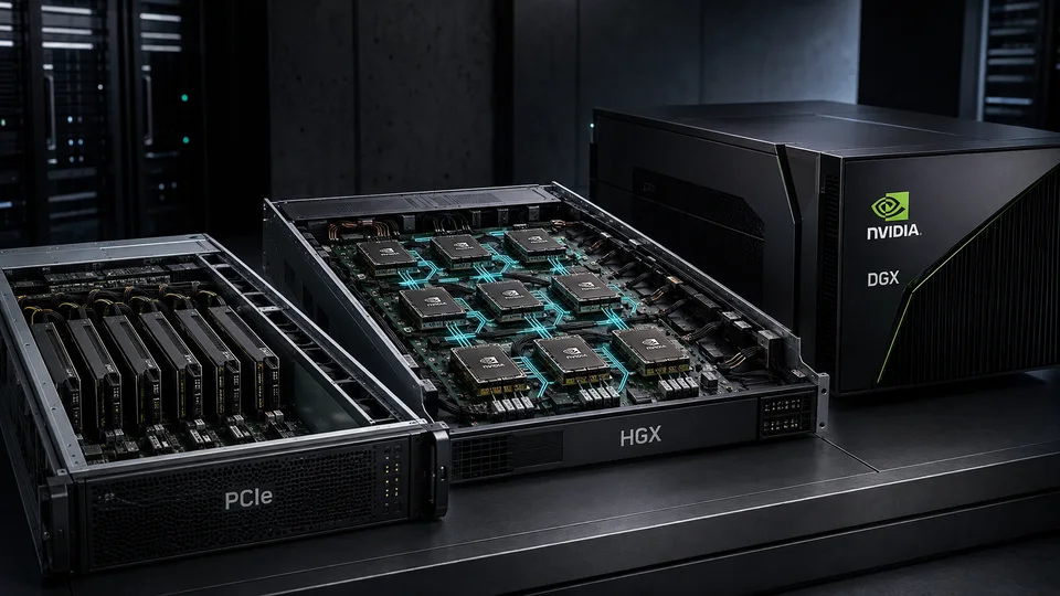
DGX, HGX or a PCIe GPU server?
Separate the need for a fast GPU fabric from the value of an integrated system, its software and its support contract.
DGX is sometimes used as if it were the technical name for any powerful GPU server. That confusion can turn into an expensive purchasing mistake. A buyer may expect a fundamentally different class of compute performance, when much of the hardware capability comes from an HGX platform that is also available inside OEM systems. The additional value of DGX lies in the complete product: its integration, software, validation and services.
The distinction is especially useful for teams serving open-weight models, building retrieval-augmented generation systems or expanding capacity gradually. Those teams need to establish both whether they need a tightly connected multi-GPU platform and whether they can make practical use of the services sold with it.
Establish what is being quoted
| Option | What it is | Principal value |
|---|---|---|
| DGX | A complete NVIDIA-branded system with hardware, DGX OS, firmware, management tools and integrated support | A validated configuration and a coordinated operational and support model |
| HGX | A multi-GPU compute platform integrated into an OEM server; in the H100/H200 examples here, SXM GPUs, a baseboard, NVLink and NVSwitch | Fast GPU-to-GPU communication for work distributed across several GPUs |
| PCIe GPU server | A server chassis fitted with PCIe add-in cards | Flexibility in card count and type, with options for incremental growth |
The DGX H100/H200 user guide describes an eight-GPU system with CPUs, memory, storage, networking and four NVSwitches. An OEM server based on the corresponding eight-GPU HGX platform can provide the same class of internal GPU fabric. The comparison must account for the complete configurations, but DGX should not be treated as “a faster HGX” simply because of its name.
Part of what a DGX purchase buys is a tested bill of materials, firmware, diagnostics, monitoring and a defined installation and support process. NVIDIA’s DGX software resources describe DGX OS as a customized Ubuntu distribution and explain that components of the software stack can also be installed on standard Ubuntu or Red Hat systems. The economic case for DGX rests on the value of that tested and supported combination.
A model catalog is not enough to justify the system
Access to NVIDIA’s models and tools is sometimes offered as a reason to buy DGX. That argument combines several different products and entitlements. The public NGC Catalog includes containers, models, SDKs and other resources. NVIDIA AI Enterprise adds a commercial software and support offering whose licensing terms need to be evaluated separately.
NVIDIA’s licensing guide lists five-year AI Enterprise subscriptions with H100 PCIe, H100 NVL and H200 NVL GPUs. Activation and the applicable GPU and certified-system conditions still matter. This does not mean that every product carrying an H100 or H200 name grants unrestricted access to every model, nor does it make DGX the only route to an included subscription. Confirm the exact SKU, entitlement, start date and support eligibility in the quote.
For a team working with open-weight models such as Llama, Qwen or Mistral, the underlying model may already be available through a public repository under its own license. An optimized container or supported runtime can reduce installation and maintenance work, but ownership of a DGX is not a general requirement for accessing those model weights.
The useful question is specific: which component of the commercial software and support offering will reduce this team’s operating cost, deployment time or service risk? A long product list does not answer it. If the service uses an existing open-source runtime and internal tooling, the proposed replacement needs a concrete benefit.
Service availability belongs in the same assessment. Registration requirements, support coverage, access to updates and the practical route for hardware returns can vary with the supplier and deployment arrangement. A service that cannot be activated or used has little operational value. Even when every service is available, paying for one the team does not need still requires justification.
HGX needs a workload case of its own
Choosing an OEM HGX system instead of DGX does not automatically make the investment appropriate. The central hardware benefit is the high-bandwidth fabric inside the server. It is useful when a single model or training job is divided across GPUs and collective operations move substantial amounts of data.
Eight independent jobs, each using one GPU, may gain little from NVSwitch. Likewise, serving a model that fits comfortably on one or two GPUs may not benefit enough from an eight-GPU fabric to justify the additional cost. The result depends on model size, concurrency, latency requirements and the execution engine—not simply on whether the application is called AI.
Frameworks such as PyTorch and vLLM, and communication libraries such as NCCL, provide mechanisms for multi-GPU execution. Economical scaling still requires an appropriate parallelism strategy, batch configuration, GPU mapping and measurement. A successful launch on eight GPUs is weaker evidence than a useful improvement in cost per completed job or served request.
Crossing the boundary between servers adds another layer. In the H100/H200 configurations discussed here, NVSwitch provides the internal GPU fabric. Multi-node execution also needs suitable NICs, a compute network, storage and software tuning. The DGX SuperPOD reference architecture treats those as distinct parts of the deployment. Large distributed training and some HPC workloads can justify that investment; independent jobs will not acquire multi-node scaling merely because the necessary cables and switches have been installed.
Choose in two stages
For inference, development, RAG and limited fine-tuning, an expandable PCIe server is often a useful baseline to test. Evaluate HGX when the actual workload needs the combined resources of several GPUs and communication between them materially affects execution time. Benchmark the proposed configurations, including the efficiency gained when moving from two GPUs to four and eight.
Then assess the complete-system offering separately. Compare DGX with supported OEM alternatives, including installation, maintenance effort, software entitlements, support coverage and the price difference. The host platform guide covers the CPU, storage and network requirements that belong in both quotes.
The purchase is justified when the workload uses the hardware capability and the operating team uses the services. Prove those two parts independently. That produces a more defensible decision than selecting a product tier first and trying to find a reason for it afterward.
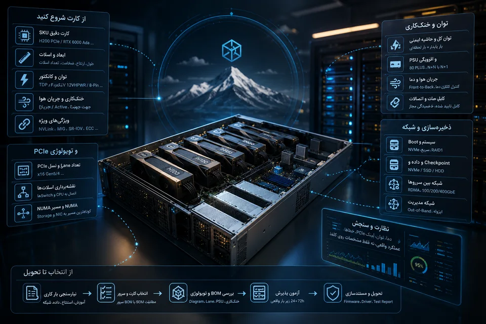
Choosing a PCIe GPU server: fit, topology, power and cooling
Check the exact GPU and server configuration, then verify sustained performance before accepting the system.
An “eight-GPU server” is a starting point for an inquiry, not a compatibility statement. The number may apply only to particular cards, power limits, risers and cooling kits. A suitable purchase specifies the exact server bill of materials and the exact GPU part numbers that will operate together.
Identify the card before choosing the chassis
Product-family names conceal important differences. H100 PCIe, H100 NVL and H100 SXM are not interchangeable. Consumer cards built around the same GPU can also vary in length, width, cooler design and connector placement. These differences affect whether the card fits, whether adjacent slots remain usable and whether the server can remove its heat.
Passive cards rely on the server to force air through their heatsinks. Many consumer cards use open-air coolers designed to circulate air inside a desktop case. An active cooler does not automatically make a card suitable for a densely packed rack chassis. Check the airflow path, inlet conditions, connector clearance and the space needed for safe cable routing.
A card occupying three or four slots may block both another GPU position and an essential network adapter. The GPU types guide explains the broader product categories, but physical compatibility is always a question about the actual part number.
Read the PCIe topology
PCIe devices can generally negotiate a common supported link generation, but that does not establish OEM qualification for a particular card and server. A physically x16 slot may also have fewer electrical lanes, or may be available only with a certain CPU or riser installed.
Ask how each GPU connects to the CPUs and whether it shares an upstream link through a PCIe switch. In a dual-socket server, record which CPU owns each GPU and NIC. This matters when the application transfers data between GPUs, performs CPU offload or uses storage and networking paths that depend on PCIe traffic.
Vendor block diagrams provide the intended topology. On a configured NVIDIA system, nvidia-smi topo -m helps inspect the visible relationships between devices. Compare that output with the proposed design and test the transfers the application actually performs. The PCIe/SXM comparison discusses when a faster GPU fabric becomes valuable.
Size power for the complete operating condition
Adding GPU power ratings is not enough to size a server. CPUs, memory, disks, NICs and fans also consume power. Include the intended operating limits, transient demand, power-supply efficiency and the redundancy policy.
An advertised redundant PSU arrangement may not preserve full compute capacity after a supply or input feed fails. Ask whether the quoted configuration maintains the required load in the specified failure condition, or whether it must reduce GPU power. The electrical provision at the rack must support the same assumptions.
Power cables and GPU enablement kits are part of the configuration. Their connectors, ratings and routing should appear in the bill of materials. Treat them as required components of the system, not accessories to resolve after the cards arrive.
Cooling must work under sustained load
Check the OEM’s supported cooling kit, ambient-temperature limits and card population rules. A configuration may support a given GPU only below a particular inlet temperature, or only with a certain fan, heatsink or blanking arrangement.
Liquid cooling introduces its own integration work: coolant distribution or radiators, pumps, maintenance and failure handling. Cooling the GPU package does not remove the need to cool memory, voltage regulators and other server components. The chosen arrangement must support the complete system.
Acceptance testing should establish that the server can sustain the intended workload without unacceptable thermal or power throttling. A short demonstration that loads the model and produces an answer does not establish stable production performance.
Provide the host resources the application uses
There is no fixed CPU-core or RAM-to-GPU ratio that fits every workload. Tokenization, image decoding, augmentation, retrieval, caching and CPU offload can each change host requirements. Start with a representative application run and measure the resources used by the planned number of concurrent jobs.
Storage needs a similar distinction between the operating system, local scratch space and persistent datasets or checkpoints. The network must then support the actual movement of that data. Choosing 10, 100 or 400 Gb/s networking by habit leaves the most important question unanswered: what traffic must cross it, and when? Distributed execution may also require an appropriate RDMA configuration and an acceptable level of network oversubscription. These components are covered in more detail in the server platform guide.
Treat comparison tables as a shortlist
A vendor’s maximum GPU count or a comparison table can narrow the field. Neither certifies the final configuration. Programs such as NVIDIA-Certified Systems are useful references, but the supported combination may depend on CPU choice, firmware, risers, GPU bridges, storage adapters, power supplies and cooling kits.
| Before placing the order | Evidence to request |
|---|---|
| Exact hardware configuration | Server and GPU part numbers, enablement kits, cables, risers and PSU arrangement |
| Official compatibility | The OEM’s supported configuration or a written confirmation covering the proposed bill of materials |
| Device topology | CPU/GPU/NIC block diagram, PCIe lane widths and any shared switch uplinks |
| Software and firmware | Proposed BIOS, BMC, GPU driver and runtime versions |
| Sustained operation | Expected power limits, inlet conditions and the acceptance workload |
| Future expansion | The additional parts and supported population rules needed for the planned upgrade |
The same standard should apply when comparing DGX, HGX and conventional PCIe systems. A product family is not a complete bill of materials.
Agree on acceptance tests before delivery
A practical acceptance run may last 24–72 hours, depending on the deployment and support agreement. Use the actual application alongside targeted hardware checks. Record temperature, clock behavior, power limits, negotiated PCIe links and any PCIe AER, NVIDIA Xid or relevant ECC errors. Where the workload spans GPUs, include its communication pattern and collective operations in the test.
If the system is designed to maintain service after a PSU or feed failure, include a controlled test of that condition under the agreed operating procedure. Verify that usable performance and power behavior match the promise in the quote.
Define what constitutes a pass before the server is delivered. The important result is a stable, supported configuration that meets the workload’s targets. That agreement makes integration responsibility explicit and prevents a buyer from discovering, after installation, that a nominally compatible set of parts still needs substantial engineering work.